5.2 A Neuron: Two ways to think about it
There have always been two motivations for artificial neural nets: to understand biological computation, and to build predictors. In a statistical learning course, we focus on the second. Biology is just for the illustration of how neural nets work:
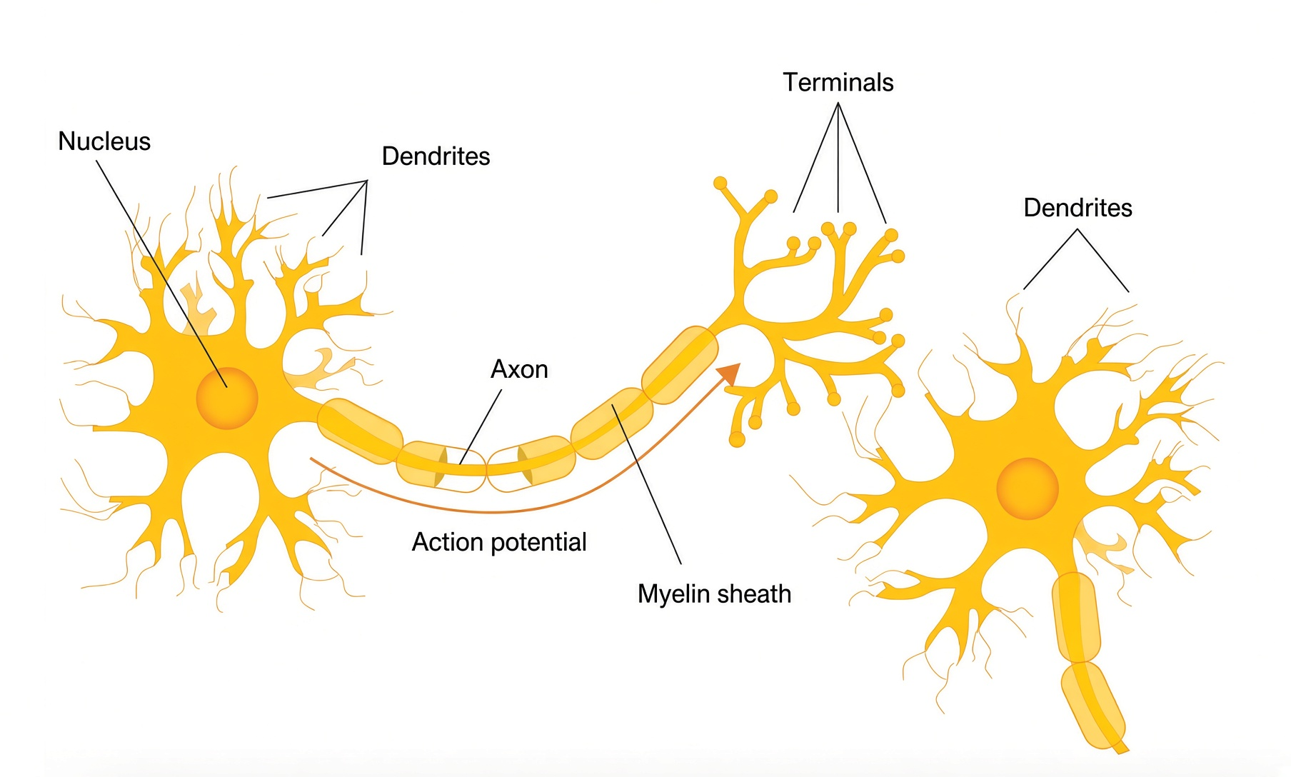
They are many simple units, densely connected, adapting in parallel.
The object we train is \(a=\sigma(w^\top x+b)\), stacked, to predict a continuous \(y\).
A Threshold Gate
McCulloch and Pitts (1943) replaced the biology with a threshold unit:
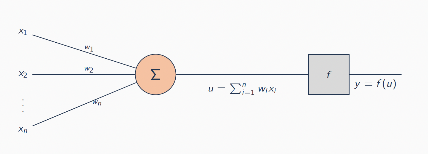
Inputs and output are bits, \[ y = \mathbf{1}_{\Bigl\{\sum_{i=1}^n w_i x_i \ge \tau\Bigr\}}, \qquad x_i,y\in\{0,1\}. \]
Networks of these units can compute any Boolean function. That is discrete universality. It does not give a real-valued \(y\), and it does not give a way to fit \(w\) from data.
The Perceptron
Rosenblatt (1958) kept the gate and added a learning rule. Predict \(\hat y=\mathbf{1}_{\{w^\top x+b\ge 0\}}\) on a labelled bit \(y\in\{0,1\}\). If the bit is right, do nothing. If it is wrong, move \(w\) parallel or anti-parallel to \(x\):
\[\begin{align*} &w \leftarrow w + \alpha\,(y-\hat y)\,x\\ &b \leftarrow b + \alpha\,(y-\hat y). \end{align*}\]
The scalar \(y-\hat y\) is \(0\), \(+1\), or \(-1\). This model introduced the idea of error-driven local change of weights. However, it is not appropriate for a continuous response, since the output is still in \(\{0,1\}\).
The Modern Unit in the Regression Framework
Replace now the bits by real-valued numbers and the hard step by a rectified linear unit (ReLU):
\[\begin{align*} z &= w^\top x + b,\\ a &= \sigma(z),\\ \sigma(z)&=\mathrm{ReLU}(z)=\max\{z,0\}. \end{align*}\]
Three choices make this a regression unit rather than a perceptron:
The coordinates of \(x\), \(w\), \(b\), and \(a\) are real.
The last layer of a network often has no \(\sigma\): we want \(\hat y=w^\top a+b\in\mathbb{R}\), free to be above or below any floor the hidden units have imposed.
We train by decreasing the MSE
\[ J=\frac1n\sum_{i=1}^n\frac12\bigl(\hat y_{i}-y_{i}\bigr)^2. \]
The factor \(1/2\) is used for scaling purposes (it will cancel a \(2\) later).
The McCulloch–Pitts step is a classifier and is not usefully differentiable. The identity \(f(z)=z\) is differentiable, but a stack of identities is one linear map — last chapter’s model with \(\phi(x)=x\). ReLU is zero on \((-\infty,0]\) and the identity on \([0,\infty)\): one corner, differentiable almost everywhere, cheap to stack. At \(z=0\) any subgradient in \([0,1]\) is valid; usually software picks \(0\) or \(1\) by convention.