10.2 Random Forests
In the regression notes we already saw the drawback of a single tree and the benefit of aggregating unstable, relatively inaccurate “weak learners” into a stronger predictor.
Bagging, boosting, and random forests all combine many trees. Bagging and random forests grow individual trees with random perturbations and then aggregate them. Boosting instead grows models sequentially, each with a small contribution, and adds them to the current fit.
10.2.1 Bagging Predictors for Classification
Draw bootstrap samples with replacement (so some observations appear more than once). Fit a CART tree to each bootstrap sample (the trees themselves may be tuned by cross-validation) and combine the \(B\) predictions by majority vote: \[ \hat{f}_{\operatorname{bag}}(x) = \operatorname{majority\ vote}\bigl\{\hat{f}_b(x)\bigr\}_{b=1}^{B}. \] Averaging in this way can reduce the variance of a single tree substantially. In the construction below, CART could be replaced by another unstable learner. The toy example compares one tree with a bagged ensemble:
# Simulate data to use for the example
set.seed(2)
n = 1000
x1 = runif(n, -1, 1)
x2 = runif(n, -1, 1)
y = rbinom(n, size = 1, prob = ifelse((x1 + x2 > -0.5) & (x1 +
    x2 < 0.5), 0.8, 0.2))
xgrid = expand.grid(x1 = seq(-1, 1, 0.01), x2 = seq(-1, 1, 0.01))

par(mfrow = c(1, 2))

# Fit CART using rpart
library(rpart)
rpart.fit = rpart(as.factor(y) ~ x1 + x2, data = data.frame(x1,
    x2, y))

# A different tree from one bootstrap sample: rpart.fit =
# rpart(as.factor(y) ~ x1 + x2, data = data.frame(x1, x2,
# y)[sample(1:n, n, replace = TRUE), ])

pred = matrix(predict(rpart.fit, xgrid, type = "class") == 1,
    201, 201)
contour(seq(-1, 1, 0.01), seq(-1, 1, 0.01), pred, levels = 0.5,
    labels = "", axes = FALSE)
points(x1, x2, col = ifelse(y == 1, "darkblue", "orange"), pch = 16,
    yaxt = "n", xaxt = "n")
points(xgrid, pch = ".", cex = 1.2, col = ifelse(pred, "darkblue",
    "orange"))
box()
title("CART")

# Fit bagging
library(ipred)
bag.fit = bagging(as.factor(y) ~ x1 + x2, data = data.frame(x1,
    x2, y), nbagg = 200)
pred = matrix(predict(bag.fit, xgrid) == 1, 201, 201)
contour(seq(-1, 1, 0.01), seq(-1, 1, 0.01), pred, levels = 0.5,
    labels = "", axes = FALSE)
points(x1, x2, col = ifelse(y == 1, "darkblue", "orange"), pch = 16,
    yaxt = "n", xaxt = "n")
points(xgrid, pch = ".", cex = 1.2, col = ifelse(pred, "darkblue",
    "orange"))
box()
title("Bagging")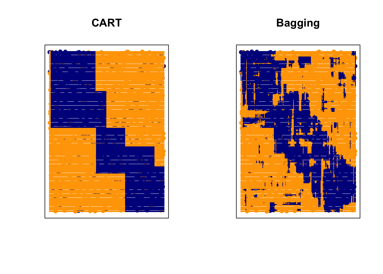
Bagging can cut the variance of unstable learners such as trees and often improves prediction. The price is interpretability: the simple rectangular structure of a single tree is lost. A second limitation is that bagged trees tend to be highly correlated, which reduces the benefit of averaging.
10.2.2 Random Forests
Random forests keep the bootstrap (or subsample) step and add extra randomness through tuning parameters. To fit a forest one must choose at least the following.
- The number of trees. A large number stabilizes the ensemble; once the estimate has settled, extra trees mainly cost computation.
- How many observations to use for each tree. With sampling with replacement one often uses a sample of size \(n\).
- The number of randomly selected predictors available at each split (
mtry). This is the main tuning parameter: larger values are more adaptive when the signal is sparse; smaller values help when predictors are highly correlated. For classification the usual default is \(\texttt{mtry}=\lfloor\sqrt{p}\rfloor\).
Splitting stops when a node has no more than nodesize observations. That role is a little like the neighborhood size \(k\) in \(k\)NN, although the effect interacts strongly with the other tuning parameters.
OOB error and the number of trees. Growing more trees does not overfit in the usual sense: after the ensemble has settled, extra trees mostly cost time. Each observation is left out of about one-third of the bootstrap samples; the votes on those left-out cases are the out-of-bag (OOB) predictions. The OOB error rate is a built-in estimate of test error, which is the main reason a forest can be used without a separate validation set.
# Generate some data with larger p
set.seed(542)
n = 1000
p = 10
X = matrix(runif(n * p, -1, 1), n, p)
x1 = X[, 1]
x2 = X[, 2]
y = rbinom(n, size = 1, prob = ifelse((x1 + x2 > -0.5) & (x1 +
    x2 < 0.5), 0.8, 0.2))
xgrid = expand.grid(x1 = seq(-1, 1, 0.01), x2 = seq(-1, 1, 0.01))

# Fit a random forest with a selected tuning
library(randomForest)

rf.fit = randomForest(X, as.factor(y), ntree = 1000, mtry = 7,
    nodesize = 10, sampsize = 800)

# Last row of err.rate is the OOB error after all trees
rf.fit$err.rate[nrow(rf.fit$err.rate), "OOB"]
## OOB
## 0.316Instead of manufacturing a test-set labeling by hand, compare the forest with the Bayes rule on a fresh sample.
# Testing data
Xtest = matrix(runif(n * p, -1, 1), n, p)

# Bayes rule for this simulation
BayesRule = ifelse((Xtest[, 1] + Xtest[, 2] > -0.5) & (Xtest[,
    1] + Xtest[, 2] < 0.5), 1, 0)

mean((predict(rf.fit, Xtest) == "1") == BayesRule)
## [1] 0.826That number is the fraction of test points on which the forest agrees with the Bayes rule, not the ordinary misclassification rate.
Variable importance
A forest (or a boosted tree model) no longer offers a single split path, but it does give a ranking of predictors. Two common scores are:
- the total decrease in impurity (Gini) attributed to splits on that variable;
- a permutation score: scramble one column in the OOB sample and record how much the OOB error rises.
##    MeanDecreaseGini
## 1          57.67159
## 2          48.22224
## 3          25.00175
## 4          23.08845
## 5          24.86713
## 6          24.75000
## 7          25.19696
## 8          22.78443
## 9          25.59233
## 10         27.78592
Large importance is not a causal claim, and correlated predictors share credit. The xgboost chunk at the end of the chapter prints a gain-based ranking of the same kind.