9.1 Linear SVM in the Separable Case: Separation Margin
We begin with the hard-margin linear classifier, the version associated with Vapnik and Chervonenkis in the 1960s and later developed into the modern SVM (Cortes and Vapnik, 1995). Assume we observe training data \(\mathcal{D}_n = \{(x_i, y_i)\}_{i=1}^{n}\), where \(x_i \in \mathbb{R}^p\) are the features and \(y_i \in \{-1,1\}\) is the class label coded as \(-1\) or \(+1\).
The goal is to estimate a real-valued function \(f(x)\) and the classification rule \(C(x) = \operatorname{sign}\{f(x)\}\). The Bayes-optimal classifier (equal misclassification costs) is
\[
C^*(x) = \operatorname{sign}\Bigl\{ P(Y=1\mid X=x) - P(Y=-1 \mid X=x) \Bigr\}.
\]
In contrast to logistic regression or DA, SVMs do not model \(P(Y\mid X)\) or the class-conditional densities \(P(X\mid Y)\). They directly model the decision boundary. The fitted score \(f(x)\) is (up to scale) a signed distance to that boundary, not a class probability. If probabilities are needed later, a common device is Platt scaling: a logistic regression of \(y\) on \(f(x)\), typically on a hold-out sample. That step is not part of the SVM itself.
9.1.1 Maximum-Margin Classifier
With labels \(y_i \in \{-1,1\}\), the classification rule based on \(f(x)\) is \[\begin{align*} \hat{y} &= +1 \quad\text{if } f(x)>0,\\ \hat{y} &= -1 \quad\text{if } f(x)<0. \end{align*}\]
The classification is correct if \(y_i f(x_i)>0\). The quantity \(y_i f(x_i)\) is the functional margin: if it is positive, the point is on the correct side; if it is negative, the point is on the wrong side. Larger positive values mean a more confident correct classification.
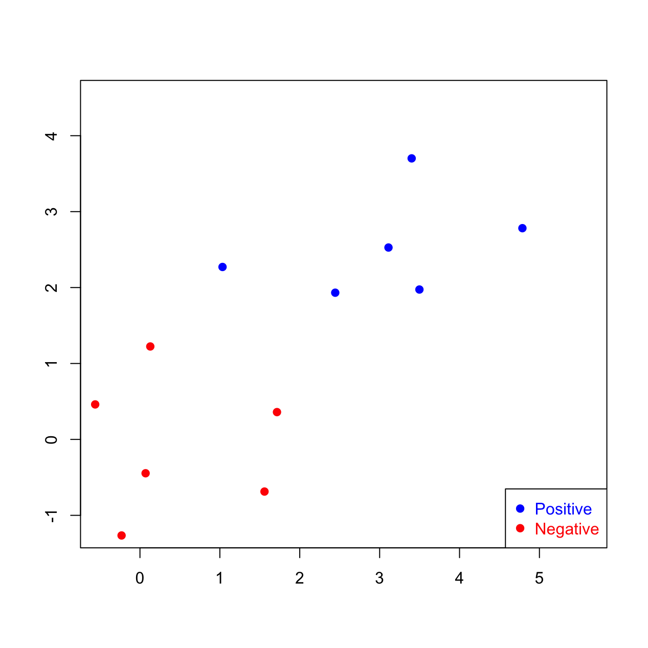
If the classes are linearly separable, we look for a linear function \(f(x) = x^T\beta + \beta_0\) that separates the two groups. Many such hyperplanes exist:
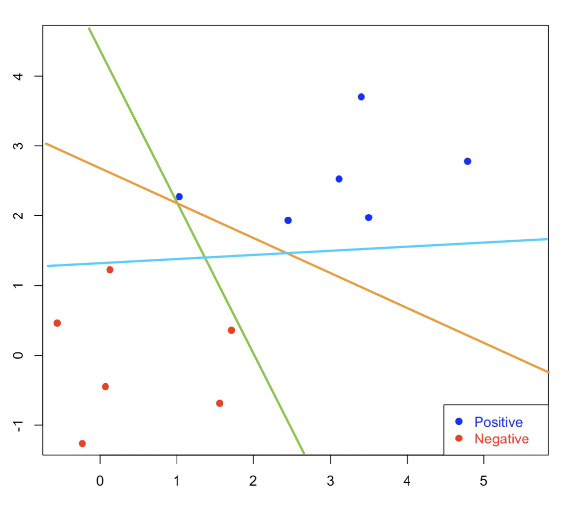
Figure 9.1: Separating lines: which one is best?
Among all these lines, which one is best?
Although many lines can perfectly separate the two classes, SVMs define the best line as the line that maximizes the separation margin, that is the width between the two dotted lines:
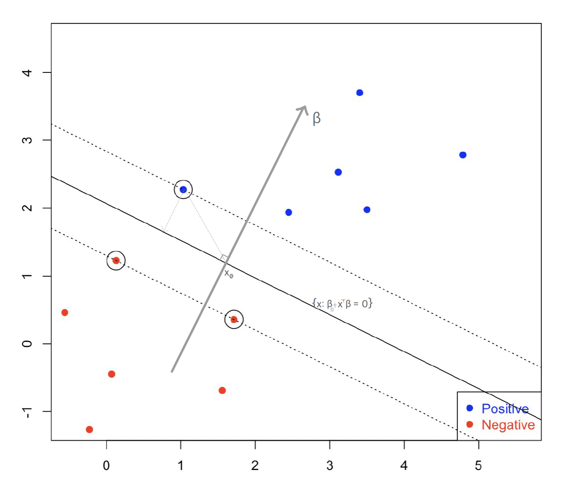
Figure 9.2: SVM: maximum-margin separating line
Mathematical Formulation
Write the linear decision function as \[ f(x) = \beta_0 + x^T\beta. \] The separating hyperplane is the level set \[ L = \bigl\{ x : \beta_0 + x^T\beta = 0 \bigr\}. \] In the separable case, every observation with \(y_i = +1\) satisfies \(f(x_i)>0\), and every observation with \(y_i = -1\) satisfies \(f(x_i)<0\).
The signed distance of a point \(x\) to the hyperplane is \[ \left\langle \frac{\beta}{\|\beta\|},\, x-x_0 \right\rangle, \] where \(x_0\in L\).
Remark. When we define a distance we usually take an unsigned version, \(|x-x_0|\) or a square, which is always nonnegative. In the SVM derivation we keep the sign, because the sign records which side of the hyperplane the point occupies. A positive signed distance means \(x\) lies on the side toward which \(\beta\) points; a negative signed distance means \(x\) lies on the opposite side.
To compute the signed distance, pick any \(x_0\in L\), so \[ f(x_0)=0 \quad\Leftrightarrow\quad x_0^T\beta = -\beta_0. \] Project \(x-x_0\) onto the unit normal \(\beta/\|\beta\|\): \[\begin{align*} \left\langle \frac{\beta}{\|\beta\|},\, x-x_0 \right\rangle &= (x-x_0)^T \frac{\beta}{\|\beta\|}\\ &= \frac{1}{\|\beta\|}\bigl(x^T\beta + \beta_0\bigr) = \frac{1}{\|\beta\|}\, f(x). \end{align*}\] Thus \(f(x)\) is proportional to the signed distance from \(x\) to \(L\). When \(\|\beta\|=1\), \(f(x)\) is that signed distance.
The goal of the SVM is to separate the two classes and maximize the distance to the closest points from either class (Vapnik, 1996), that is, to construct the maximum margin:
\[ \max_{\beta,\,\beta_0,\,\|\beta\|=1} M \] \[ \text{subject to }\quad y_i\bigl(x_i^T\beta + \beta_0\bigr) \ge M,\qquad i=1,\ldots,n. \]
Every training point is then at least a signed distance \(M\) from the decision boundary. Equivalently, if \(y_i=+1\) we require \(f(x_i)\ge M\), and if \(y_i=-1\) we require \(f(x_i)\le -M\). Maximizing the minimum distance is exactly maximizing the margin.
The constraint \(\|\beta\|=1\) is inconvenient because the geometric margin also depends on the scale of \(\beta\). Dropping the unit-norm restriction, the same requirement can be written \[ \frac{1}{\|\beta\|}\, y_i\bigl(x_i^T\beta + \beta_0\bigr) \ge M. \] The scale of \(\beta\) is now free, so we may set \(\|\beta\|=1/M\) and rewrite the problem as\[ \min_{\beta,\,\beta_0}\ \frac12\|\beta\|^2 \] \[ \text{subject to }\quad y_i\bigl(x_i^T\beta + \beta_0\bigr) \ge 1,\qquad i=1,\ldots,n. \]
This constraint says that every point is at least \(1/\|\beta\|\) away from the separating plane and lies on the correct side of the corresponding margin line: \[ \begin{cases} x_i^T\beta + \beta_0 \ge 1, & \text{if } y_i = +1,\\ x_i^T\beta + \beta_0 \le -1, & \text{if } y_i = -1. \end{cases} \] The full margin width between the two dotted lines is \(2/\|\beta\|\).
If \(x_i\) lies on one of the dotted lines, that is, if \(y_i(x_i^T\beta+\beta_0)-1=0\), the \(i\)th constraint is active. If \(y_i(x_i^T\beta+\beta_0)-1>0\), it is inactive. At the optimum there must be at least two active points, one from each class; otherwise the margin could be widened.
This is the primal form of the hard-margin SVM:
Primal form (hard margin)
\[ \operatorname{minimize}_{\beta,\,\beta_0}\quad \frac12\|\beta\|^2 \] \[ \text{subject to }\quad y_i\bigl(x_i^T\beta+\beta_0\bigr)\ge 1,\qquad i=1,\ldots,n. \]
The max-margin problem is a convex quadratic program with linear inequality constraints, so it has no local-optima issues as a mathematical program. Feature scaling, a barely separable sample, and solver tolerances can still give a poor numerical fit. This primal is feasible only in the perfectly separable case.
9.1.2 The KKT Conditions: From the Primal to the Dual
Statistically, the SVM is regularized hinge loss: \(\sum_i(1-y_i f(x_i))_+ + \lambda\|\beta\|^2\), with \(\lambda=1/C\). We derive the dual because that program is equivalent to the hinge problem and because the dual depends on the data only through inner products \(x_i^T x_j\). The quadratic program over \(\alpha\) is the algorithm; the loss-plus-penalty criterion is the definition. We will return to that view after the kernels.
The Karush–Kuhn–Tucker (KKT) conditions are necessary conditions for optimality in constrained problems (and they are sufficient here because the program is convex). We review the idea briefly, then apply it to the SVM.
With no constraints, a minimum of a differentiable function \(f\) requires \(\nabla f(x)=0\): there is no direction in which \(f\) can still decrease.
Equality-Constrained Optimization
Now minimize \(f(x)\) subject to \(h(x)=0\). The feasible set is \(\mathcal{S}=\{x:h(x)=0\}\). At a constrained minimum the gradient of \(f\) need not vanish, but any descent direction of \(f\) must be forbidden by the constraint: it must leave \(\mathcal{S}\). That is expressed by \[ \nabla f(x) + \lambda\,\nabla h(x) = 0,\qquad \lambda\in\mathbb{R}. \] Equivalently, the Lagrangian \[ \mathcal{L}(x,\alpha) = f(x) + \alpha\, h(x) \] is stationary in \(x\). Here \(\alpha\) is a Lagrange multiplier. Geometrically, \(\nabla h(x)\) is orthogonal to the constraint surface. At a constrained local minimum, \(\nabla f\) must be orthogonal to that surface as well, so \(\nabla f\) and \(\nabla h\) are parallel: \[ \nabla f(x^*) = -\alpha\,\nabla h(x^*). \]
Inequality-Constrained Optimization
Consider\[ \operatorname{minimize}_{x}\ g(x) \qquad\text{subject to}\quad h_i(x)\le 0,\quad i=1,\ldots,n. \]
\[ \mathcal{L}(x,\alpha) = g(x) + \sum_{i=1}^{n} \alpha_i h_i(x),\qquad \alpha_i\ge 0. \]
Two nested problems are associated with \(\mathcal{L}\):
The primal problem, \[ \min_{x}\ \max_{\alpha\ge 0}\ \mathcal{L}(x,\alpha). \] If \(x\) violates a constraint, \(h_i(x)>0\), we can send \(\alpha_i\to\infty\) and make \(\mathcal{L}\) arbitrarily large. Hence the inner maximization is finite only for feasible \(x\).
The dual problem, \[ \max_{\alpha\ge 0}\ \min_{x}\ \mathcal{L}(x,\alpha). \]
In general \[ \underbrace{\max_{\alpha\ge 0}\min_{x}\mathcal{L}(x,\alpha)}_{\text{dual}} \ \le\ \underbrace{\min_{x}\max_{\alpha\ge 0}\mathcal{L}(x,\alpha)}_{\text{primal}}. \] Equality holds (strong duality) when \(g\) and the \(h_i\) are convex and a mild feasibility condition is satisfied. Both conditions hold for the SVM.
\[ \min_{\beta,\,\beta_0}\ \frac12\|\beta\|^2 \] \[ \text{subject to }\quad -\bigl\{y_i(x_i^T\beta+\beta_0)-1\bigr\}\le 0,\qquad i=1,\ldots,n. \]
The Lagrangian is \[ \mathcal{L}(\beta,\beta_0,\alpha) = \frac12\|\beta\|^2 - \sum_{i=1}^{n}\alpha_i\bigl\{y_i(x_i^T\beta+\beta_0)-1\bigr\}, \qquad \alpha_i\ge 0. \] We solve the dual: first minimize \(\mathcal{L}\) in \((\beta,\beta_0)\), then maximize in \(\alpha\).
9.1.3 Solving the Dual Problem
Stationarity in \(\beta\) and \(\beta_0\) gives \[\begin{align*} \nabla_{\beta}\mathcal{L}=0 &\quad\Leftrightarrow\quad \beta = \sum_{i=1}^{n}\alpha_i y_i x_i,\\ \nabla_{\beta_0}\mathcal{L}=0 &\quad\Leftrightarrow\quad \sum_{i=1}^{n}\alpha_i y_i = 0. \end{align*}\] Substitute these relations back into \(\mathcal{L}\) to obtain the dual objective \[ \mathcal{L}(\alpha) = \sum_{i=1}^{n}\alpha_i - \frac12\sum_{i=1}^{n}\sum_{j=1}^{n} y_i y_j\alpha_i\alpha_j\, x_i^T x_j. \] The dual problem is therefore \[ \max_{\alpha}\ \sum_{i=1}^{n}\alpha_i - \frac12\sum_{i,j=1}^{n} y_i y_j\alpha_i\alpha_j\, x_i^T x_j \] \[ \text{subject to }\quad \alpha_i\ge 0,\quad i=1,\ldots,n, \qquad \sum_{i=1}^{n}\alpha_i y_i=0. \] This is again a convex quadratic program. Complementary slackness implies that if a point is inactive (strictly on the correct side of its margin line), then \(\alpha_i=0\). The points with \(\alpha_i>0\) are the support vectors. Only they enter the expansion of \(\hat\beta\).
Linear SVM algorithm (hard-margin dual)
- Solve the dual for \(\hat\alpha\).
- Recover \[ \hat\beta = \sum_{i=1}^{n}\hat\alpha_i y_i x_i. \]
- Recover \(\hat\beta_0\) from any support vector, using \(y_i(x_i^T\hat\beta+\hat\beta_0)=1\). In the hard-margin case we can also take the midpoint of the two closest support vectors from opposite classes:
\[
\hat\beta_0
= -\frac12
\Bigl(
\max_{i:y_i=-1} x_i^T\hat\beta
+ \min_{i:y_i=+1} x_i^T\hat\beta
\Bigr).
\]
This midpoint formula is for the hard-margin problem only. Once slack is allowed, the closest points need not lie on the margin. In
e1071the intercept used in the plots is-rhofrom the solver. - For a new \(x\), predict \(\operatorname{sign}(x^T\hat\beta+\hat\beta_0)\).
Remarks
Linear separability means that many hyperplanes classify the training data perfectly. The SVM selects the one with the largest margin. The primal constraints enforce correct classification with a functional margin of at least one. In the dual, the Lagrange multipliers \(\alpha_i\) are nonzero only for points that sit on the margin. Those points are the support vectors: if they were removed, the fitted hyperplane would change. All other training points can be moved (a little) or even deleted without affecting \(\hat f\).