6.2 Regression Forests
Regression forests extend a single tree by combining many trees into an ensemble. Two sources of randomness are used. First, each tree is grown on a bootstrap sample of the observations (bagging). Second, in a random forest, each split searches only a random subset of the \(p\) predictors. The extra randomness makes the trees less correlated. The ensemble prediction is the average of the individual trees, which typically lowers variance relative to one deep tree and improves accuracy and stability. The simple picture of a single tree is lost.
6.2.1 Weak and Strong Learners
Single trees have two familiar drawbacks: they are unstable – small changes in the data can produce very different trees – and they often lack accuracy. In that sense a single tree is a weak learner.
A standard response is to combine many weak learners into a strong learner. Ensemble methods of this type include bagging, random forests, and boosting.
Bagging and random forests grow trees under different random perturbations and average their predictions. Boosting is sequential: it progressively fits simple models and adds them together.
Conceptually, an ensemble of trees looks like this: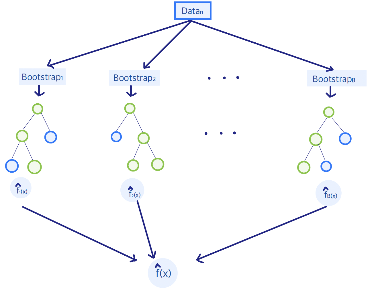
6.2.2 Bootstrap Aggregation (Bagging)
Bagging (bootstrap aggregation) is an ensemble method designed to reduce the variance of unstable predictors. It repeatedly resamples the training data with replacement, fits a model on each bootstrap sample, and averages the predictions (regression) or takes a majority vote (classification).
Write the training data as \(\mathbf{Z} = \bigl\{(x_i, y_i): i=1,\ldots,n \bigr\}\). Draw bootstrap samples \(\mathbf{Z}^{*b} = \bigl\{(x_i^{*b}, y_i^{*b}): i=1,\ldots,n \bigr\}\) for \(b=1, \ldots, B\), \[\begin{align*} \mathbf{Z}^{*1} &: (x_1^{*1}, y_1^{*1}), (x_2^{*1}, y_2^{*1}), \ldots, (x_n^{*1}, y_n^{*1})\\ \mathbf{Z}^{*2} &: (x_1^{*2}, y_1^{*2}), (x_2^{*2}, y_2^{*2}), \ldots, (x_n^{*2}, y_n^{*2})\\ \vdots &\\ \mathbf{Z}^{*B} &: (x_1^{*B}, y_1^{*B}), (x_2^{*B}, y_2^{*B}), \ldots, (x_n^{*B}, y_n^{*B}). \end{align*}\]
Fit \(\hat{f}^{*b}\) on \(\mathbf{Z}^{*b}\). The bagging estimate is \[\hat{f}_{\mathrm{bag}}(x) = \frac{1}{B} \sum_{b=1}^{B} \hat{f}^{*b}(x).\]
Averaging many trees can cut variance substantially. Two caveats: the readable structure of one tree is lost, and if the trees stay highly correlated the variance reduction is limited.
6.2.3 Random Forests
Random forests grew out of several 1990s ideas. Breiman’s bagging showed that averaging unstable predictors such as trees can reduce variance. Ho’s random subspace method (1998) showed that further diversity is available by training each tree on a random subset of features. Breiman combined the two in random forests: bagging plus a random subset of predictors at every split. The result is a large collection of de-correlated trees whose average is typically both more accurate and more stable than a single tree.
The algorithm has a few moving parts:
Bootstrap sampling (bagging): each tree is grown on a bootstrap sample of the training data.
Random feature selection: at each split, only a random subset of the \(p\) features is eligible. That extra randomness decorrelates the trees and improves the variance reduction from averaging.
Tree growth: forest trees are usually grown deep and not pruned, so that each tree can be highly flexible. Overfitting of any one tree is less of a concern because the average stabilizes the fit.
Prediction: for regression, average the \(B\) tree predictions.
Out-of-bag (OOB) error: each bootstrap sample leaves out about one-third of the rows. Those left-out observations give a built-in estimate of prediction error, close in spirit to cross-validation.
Sketch of the Algorithm
For \(b=1, \ldots, B\)
Draw a bootstrap sample of size \(n\), \(\mathbf{Z}^{*b}\), from the training data.
Grow a large tree \(T_b\) by repeating the following steps at each terminal node until a minimum node size is reached:
1. Select $m$ variables at random from the $p$ variables.

2. Pick the best variable and split-point among those $m$.

3. Split the node into two children.
Output the forest \(\{T_b\}_{b=1}^{B}\).
Predict at a new point \(x\) (regression) \[ \hat{f}^B (x) = \frac{1}{B} \sum_{b=1}^{B} T_b(x).\]
Restrictions
At every split, a subset of \(m\) features is drawn from the \(p\) available features, and the best split is chosen only among those \(m\). A common rule of thumb is \(m=\sqrt{p}\) for classification and \(m=p/3\) for regression.
Restricting the candidate features makes it less likely that every tree leans on the same strong predictors, which lowers correlation among trees and helps the average.
6.2.4 Out-of-Bag (OOB) Samples
Out-of-bag samples are the observations that do not appear in \(\mathbf{Z}^{*b}\) and so are not used to grow \(T_b\). They are a natural test set for that tree. The OOB error aggregates, for each observation \(i\), only the trees that did not train on \(i\). Packages such as randomForest report predictions and error rates from this calculation. The estimate is typically close to \(K\)-fold cross-validation.
6.2.4.1 Variable Importance
Two common measures:
Reduction in RSS (impurity): each split records the drop in RSS and attributes that drop to the variable used. Sum those drops over all splits in a tree, then average over trees. This measures how much the variable is used to reduce training error. It tends to favor variables that offer many candidate cutpoints (numeric variables, or factors with many levels).
Permutation of predictors: for each tree \(T_b\), compute the OOB prediction error (MSE for regression). Randomly permute predictor \(j\) in the OOB data and recompute the error. The increase is a measure of importance for \(j\). Average the increase over trees;
randomForestcan also divide by the standard deviation of those increases (a scaled importance). Permutation importance can be misleading when predictors are highly correlated: the forest may split on one of several substitutes, and permuting a single \(j\) then understates the role of the group.
6.2.5 Boosting Trees
Boosting also builds an ensemble of trees, but the trees are grown sequentially. Each new tree is aimed at the errors of the current fit, rather than at a fresh bootstrap sample.
Write an additive model \[F(x) = f_1(x) + f_2(x) + \ldots + f_T(x).\] Fitting all \(T\) terms at once is hard. Forward stagewise fitting adds one term at a time. For squared error, tree \(t\) is fit to the current residuals and then added with a learning rate \(\lambda\): \[ F_t(x) = F_{t-1}(x) + \lambda\,\hat h_t(x). \] Small \(\lambda\) and a large \(T\), with \(T\) chosen by cross-validation, is the usual regularization.
Boosting often predicts better than bagging, and it can capture complex nonlinear structure. It is more sensitive to noise and outliers than bagging, and the hyperparameters (n.trees, shrinkage, tree depth) need more care.