6.1 Single-Tree Building
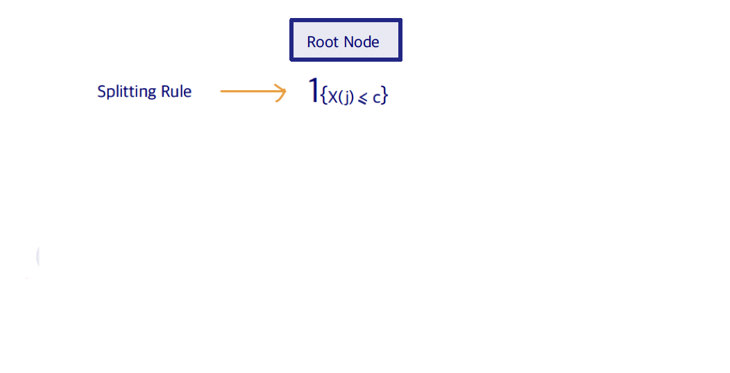
As we discussed, to build a single tree one recursively partitions the predictor space. Start by initializing the root with all of the training data. Then choose a splitting rule consisting of a predictor \(X_j\) and a constant \(c\) that splits the observations in the node: \[\mathbf{1}_{\{X_j \leq c\}}\]
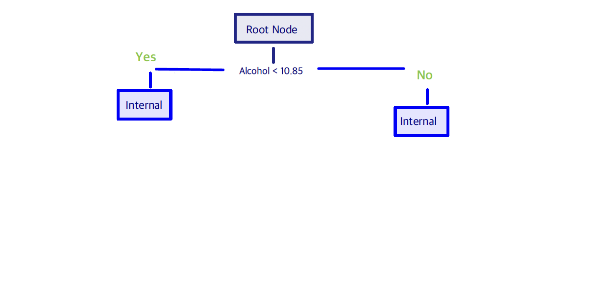
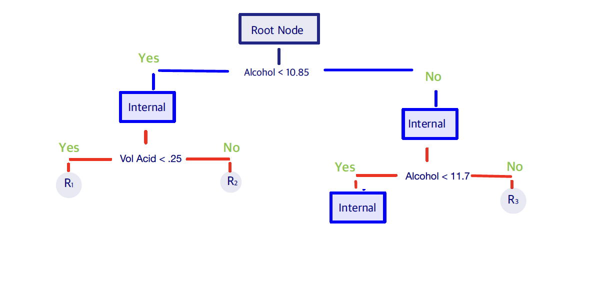
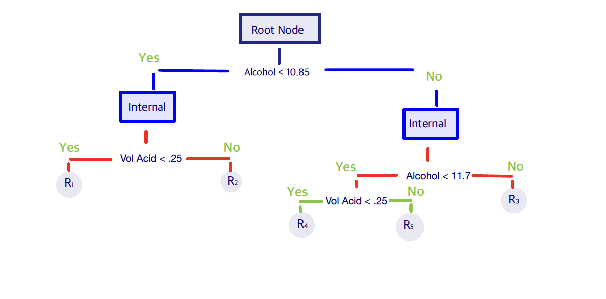
We denote a node by \((t)\) and its children by \((t_L, t_R)\). A split is a pair (variable \(j\), cutpoint \(s\)), and the procedure ends at the leaves (terminal nodes).
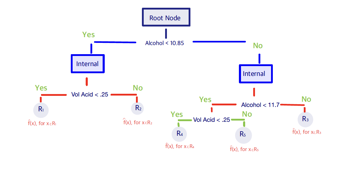 When we stop, we predict in each terminal node using the data in that node. Every leaf (a rectangular region \(R_m \subset \mathcal{X}\)) is assigned a constant, so a regression tree has the form
\[\hat{f}(X) = \sum_m c_m \mathbf{1}_{\{X \in R_m\}}.\]
The natural questions are:
- Where to split the tree?
- When to stop?
- How to predict the response at each leaf node?
6.1.1 Prediction at Leaf Nodes
Each leaf corresponds to a region \(R_m\) that contains some training points. The prediction in that leaf is the average of the response \(Y\) for the observations in \(R_m\), \(m=1, \ldots, M\): \[\hat{f}(X) = \sum_{m=1}^{M} c_m \mathbf{1}_{\{ X \in R_m\}}.\] The constants \(c_m\) are chosen by minimizing squared error in the leaf: \[\min_{c_m} \sum_{i:\, x_i \in R_m} (y_i - c_m)^2.\] The minimizer is the average of those \(y_i\) with \(x_i \in R_m\).
6.1.2 Split Criterion
Finding a global partition of \(\mathcal{X}\) with minimum residual sum of squares is computationally infeasible, so we use a greedy algorithm. This search is not guaranteed to find the piecewise-constant fit with globally smallest RSS; it only chooses the best single split at the current node. Start with all of the data at the root. A split variable \(j\) and split point \(s\) produce the half-planes \[R_1 (j,s) = \bigl\{X: X_j \leq s \bigr\} \quad \text{ and } \quad R_2 (j,s) = \bigl\{X: X_j > s \bigr\}.\] We then choose the pair \((j,s)\) that solves \[\min_{j,s} \Bigl[ \min_{c_1} \sum_{x_i \in R_1(j,s)} (y_i - c_1)^2 + \min_{c_2} \sum_{x_i \in R_2(j,s)} (y_i - c_2)^2 \Bigr].\] For any fixed \(j\) and \(s\), the inner minimization is solved by \[ \hat{c}_1 = \mathrm{ave} \bigl(y_i : x_i \in R_1(j,s) \bigr) \, \text{ and } \hat{c}_2 = \mathrm{ave} \bigl(y_i : x_i \in R_2(j,s) \bigr).\]
For each splitting variable, the best cutpoint \(s\) can be found quickly by scanning the ordered unique values, so searching over all pairs \((j,s)\) is feasible.
The same idea can be written as a split criterion \(\Phi(j,s)\), here the reduction in RSS. Regression trees are grown top-down and greedily:
Start at the root and consider
a. all variables \(j=1, \ldots, p\) and
b. all candidate split values,
c. and pick the split with the best \(\Phi\).
The data in the node are then sent to a left child and a right child.
Repeat the procedure in each child.
Split Criterion \(\Phi(j, s)\)
Reduction in RSS if we split the samples at node \(t\) into \(t_L\) and \(t_R\): \[ \Phi(j, s) = RSS(t) - \Bigl[RSS(t_R) + RSS(t_L) \Bigr] \] where \[RSS(t) = \sum_{x_i \in t} (y_i - c_t)^2, \quad \text{ with } \quad c_t = \mathrm{ave}\{y_i : x_i \in t\}.\]
Note that \(\Phi(j, s) \ge 0\), with equality if and only if the two child means are equal.
Categorical Predictors
A categorical predictor with \(m\) levels can be used directly as a split variable. In principle there are \(2^{m-1}-1\) ways to assign the \(m\) labels to the left and right child. That search is feasible only for small \(m\).
For regression with squared error there is a shortcut: order the \(m\) levels by their mean response, then treat the variable as if it were ordered. Only the \(m-1\) adjacent cuts need to be checked, and the best of those is the best binary partition of the labels.
Missing Predictor Values
Tree algorithms can handle missing predictors without discarding whole rows, which would otherwise shrink the training set quickly.
One approach is to evaluate the split using only the observations with \(X_j\) observed. After a split \((j,s)\) is chosen, missing \(X_j\) can be filled in by an imputation rule.
A more specifically CART-style option is to build surrogate splits: other variables (and a majority rule) that predict the event \(\{X_j \le s\}\). An observation missing \(X_j\) is sent left or right by the best available surrogate, then the next, and so on.
6.1.3 Single-Tree Pruning
We have a leaf prediction and a split criterion. What remains is when to stop, which determines how large the tree is.
For a binary tree write \(|T|\) for the number of terminal nodes (leaves). The number of splits is then \(|T|-1\). A large tree can overfit, but a small tree may miss structure that only appears after a weak first split. Balancing fit and size is the same “loss + penalty” idea as in penalized regression.
One possible rule is to split a node only if the decrease in RSS exceeds a certain threshold. That rule is short-sighted: a split that looks useless now may be followed by a valuable split below. The standard strategy is therefore to grow a large tree and then prune.
We start by growing a very large tree \(T_{\max}\):
until all terminal nodes are nearly pure, that is, the variability of \(Y\) in the node is small;
or until the number of observations in each terminal node is below a threshold;
or until the tree reaches a prescribed size.
The exact size of \(T_{\max}\) is not critical as long as the tree is large enough.
Notation
Subtree \(T' \preceq T\): any tree obtained from \(T\) by pruning, i.e. by collapsing some branches. Branch at node \((t)\): \(T_t\)
For any subtree \(T \preceq T_{\max}\) define the complexity cost \[R_{\alpha}(T) = R(T) + \alpha|T|,\] where \(R(T)\) is the RSS of \(T\), \(|T|\) is the number of leaves, and \(\alpha \ge 0\) is the cost of a leaf. For each fixed \(\alpha\) let \[\begin{align*} T(\alpha) &= \arg\min_{T\preceq T_{\max}} R_{\alpha}(T) \\ &= \arg\min_{T\preceq T_{\max}} \Bigl[ R(T) + \alpha|T|\Bigr]. \end{align*}\] If several trees attain the minimum, take the smallest; that subtree \(T^{*}(\alpha)\) is unique. We do not pick \(\alpha\) by minimizing \(R_{\alpha}\) on the training data. We compute the path \(T^{*}(\alpha)\) and choose \(\alpha\) by cross-validation.
For a pair of sister leaves \((t_L, t_R)\) there is a critical value \(\alpha^{*}\) such that
for any \(\alpha \ge \alpha^{*}\), we prefer to collapse them back to the parent \(t\);
for any \(\alpha \le \alpha^{*}\), we prefer to keep the two leaves.
So \(\alpha^{*}\) is the highest price we are willing to pay to keep that split. The same calculation extends to a whole branch \(T_t\). Using only the samples that fall in \(t\),
the cost of keeping the branch is \[R_{\alpha}(T_t) = R(T_t) + \alpha |T_t|;\]
the cost of cutting the branch (making \(t\) a leaf) is \[R_{\alpha}(\{t\}) = R(\{t\}) + \alpha.\]
Equating the two costs gives \[\alpha^{*} = \frac{R(\{t\}) - R(T_t)}{|T_t|-1}.\] If the working value of \(\alpha\) exceeds this \(\alpha^{*}\), the branch is too expensive and \(t\) becomes a leaf.
Searching every subtree of \(T_{\max}\) would be expensive, but it is unnecessary. Weakest-link pruning removes the least valuable branch at each step and produces a nested sequence of trees – the cost-complexity path. That path is what cptable and plotcp display later in rpart.
Weakest Link Pruning Algorithm
Start with \(T_0=T_{\max}\) and \(\alpha_0=0\).
For any non-leaf node \(t\), \[\alpha(t) = \text{ the maximal price you would pay to keep } T_t. \]
\(\alpha_1 = \min_t \alpha(t)\) The corresponding non-terminal node \(t_1\) is called the weakest link.
Cut the branch at \(t_1\).
Update the maximal price for each non-leaf node (only the ancestors of \(t_1\) change).
Find \(\alpha_2\) and cut the branch at the next weakest link.
Keep doing this until only the root remains.
The algorithm produces the nested path \[ T_{\max} = T_0 \succ T^{*}(\alpha_1) \succ T^{*}(\alpha_2) \succ \ldots \succ \{\text{root node}\}\] \[0=\alpha_0 <\alpha_1 <\alpha_2 < \ldots\] All \(\alpha \ge 0\) fall into \(m+1\) intervals \[\begin{align*} I_0 &= [0, \alpha_1)\\ I_1 &= [\alpha_1, \alpha_2)\\ \vdots &\\ I_m &= [\alpha_m, \infty) \end{align*}\] and every \(\alpha \in I_i\) shares the same optimal subtree \(T^{*}(\alpha_i)\).
Tuning of the hyperparameter \(\alpha\)
Use \(K\)-fold cross-validation to choose \(\alpha\). Grow \(T_{\max}\) on the full training data and compute the intervals \(I_0, I_1, \ldots, I_m\). Representative values in those intervals are \[\begin{align*} \beta_0 &= 0\\ \beta_1 &= \sqrt{\alpha_1 \alpha_2}\\ \vdots &\\ \beta_{m-1} &= \sqrt{\alpha_{m-1} \alpha_m}\\ \beta_m &= \infty, \end{align*}\] so each \(\beta_j\) stands for \(I_j\).
For \(K\)-fold CV, partition the data into \(K\) folds and repeat \(k=1, \ldots, K\). On the data with fold \(k\) held out, grow a large tree and extract the path \[T_0 \succ T^{*}(\beta_1) \succ \ldots \succ T^{*}(\beta_m) \succ \{\text{root node} \}.\] Compute the prediction error of each of those trees on fold \(k\). Average over folds to obtain a CV curve in \(\alpha\), and pick \(\alpha_{\min}\) or \(\alpha_{1\mathrm{se}}\).