12.2 \(K\)-means Clustering
Consider an enlarged optimization problem
\[\min_{C, \{m_k\}_{k=1}^{K}} \sum_{k=1}^{K} \sum_{C(i)=k} ||x_i - m_k||^2\]
We solve this with respect to both: the cluster function \(C(\cdot)\) and the cluster centers \(m_k\), \(k=1,\ldots, K\). But, this problem is NP-hard for \(\geq 2\) dimensions and a combinatorial algorithm is too expensive.
We could instead consider an algorithm that alternatively updates the two components:
\(C\) the cluster assignments
\(\{m_k\}_{k=1}^{K}\) the cluster means
So, we can achieve this by first fixing \(C\), and then finding the best \(\{m_k\}_{k=1}^{K}\), and second by fixing \(\{m_k\}_{k=1}^{K}\), and then finding the best \(C\). Specifically, in \(K\)-means Clustering, we need to alternate between the following two steps until convergence:
Fix \(C\), i.e. the cluster label of each subject is known. Then, for any set \(\{i : C(i) = k\}\), we only need to find the mean \[m_k = \arg \min_m \sum_{C(i)=k} ||x_i-m||^2\] which boils down to simply finding the mean within cluster \(k\), i.e. \[m_k = \frac{\sum_{C(i)=k} x_i}{\sum_i \mathbf{1}_{\{C(i)=k\}}} \]
Fix the cluster means \(\{m_k\}_{k=1}^{K}\). Then, to find the new cluster assignments, we simply recalculate the distance from an observation to each of the cluster means: \[C(i) = \arg \min_{k\in \{1, \ldots, K\}} d(x_i, m_k) \] Hence each point will be assigned to the closest cluster mean.
The \(K\)-means Clustering Algorithm can be summarized as follows:
\(K\)-means Clustering Algorithm
Randomly split the data set into \(K\) different subsets. Assign each subset a cluster label. Then iterate between (2) and (3):
Given the cluster assignment \(C\), calculate the cluster mean vectors \(m_1, \ldots, m_K\).
Given the current set of means \(\{m_1, \ldots, m_K\}\), assign each observation to the closest current cluster mean.
Stop the algorithm when \(C\) does not change.
Below is an illustration of the way the algorithm works in a toy example
Illustration of \(K\)-Means Clustering
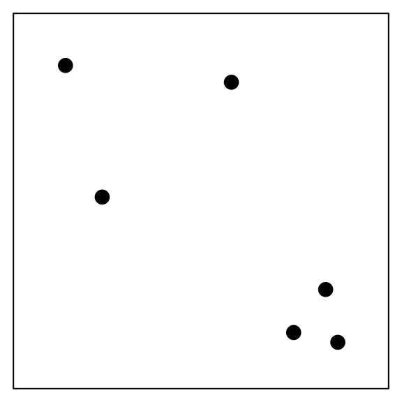
Suppose we have a set of six observations.
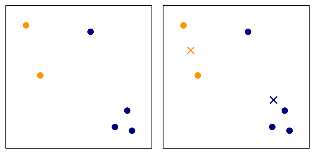
We first randomly assign them into two clusters (initiate a random \(C\) function). Based on this cluster assignment, we can calculate the corresponding cluster mean \(m_k\)’s:
Then we will assign each observation to the closest cluster mean. In this example, only the blue point on the top will be moved to a new cluster. Then the cluster means can then be recalculated.
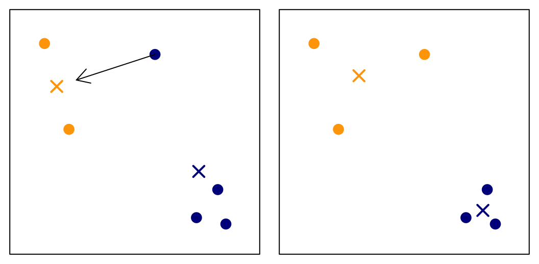
When there is nothing to move anymore, the algorithm stops. Keep in mind that we started with a random cluster assignment, and this objective function is not convex which implies that we may obtain different results if we start with different values. The solution is to try different starting points and use the best final results. This can be tuned using the nstart parameter in the kmeans() function.
# some random data
set.seed(1)
mat = matrix(rnorm(1000), 50, 20)

# if we use only one starting point
kmeans(mat, centers = 3, nstart = 1)$tot.withinss
## [1] 885.8913# if we use multiple starting points and pick the best one
kmeans(mat, centers = 3, nstart = 100)$tot.withinss## [1] 883.8241Note that the clusters are typically initialized randomly. However, this algorithm does not guarantee a global minimum, although it still leads to a local minimizer.
Two modeling assumptions are easy to miss and matter in practice. First, \(K\)-means with Euclidean (or squared Euclidean) distance treats every coordinate as comparable, so features should be put on a common scale before clustering; otherwise a variable measured in thousands will dominate one measured in fractions. Second, minimizing \(\sum \|x_i-m_k\|^2\) favors compact, roughly spherical clusters of similar size. Elongated or unequal-variance groups will be split or merged for reasons that have nothing to do with “natural” labels.
The same squared-error criterion will reappear in the next chapter: \(K\)-means is a hard-assignment, equal-covariance version of EM for a Gaussian mixture. That is the hinge between geometric clustering and model-based clustering.
An alternative approach is the \(K\)-medoids method. We need to replace the first step (updating the centers) by searching for the one observation that minimizes the distance to all others in the cluster, i.e. \[i^*_k = \arg \min_{i:C(i)=k} \sum_{C(i')=k} d(x_i, x_{i'})\] Then we use \(x_{i^*_k}\) as the ``center’’ of cluster \(k\). The assignment step is unchanged: each point is assigned to the closest medoid.
12.2.1 Categorical Variables in Clustering
By design, the \(k\)-means method cannot handle categorical variables as is unless we change them to numerical, e.g., using one-hot encoding, or ordinal encoding. Alternatively, we may also use distance metrics that are specifically designed for categorical data, e.g., Hamming distance, or the Jaccard distance.
We can also choose clustering algorithms that support categorical variables, such as \(K\)-Modes or \(K\)-prototypes.
12.2.2 Tuning \(K\)-Means: How to Choose \(K\)
When using \(K\)-Means, we need to identify an appropriate value for the number of clusters, \(k\). Some of the available methods, include:
Gap Statistics
Silhouette Statistics
Prediction Strength
When identifying the appropriate number of clusters, we need to consider a measure of compactness/tightness of clusters. A measure that quantifies the compactness or tightness of clusters can be computed based on
\[SS(K) = \sum_{k=1}^{K} \sum_{C(i)=k} ||x_i - m_k||^2 \]
A smaller SS indicates tighter clusters. As the number of clusters (\(K\)) increases, the SS inherently decreases for the same data set which means that relying only on SS can be misleading when selecting the optimal \(K\).
Gap Statistic
The gap statistic (Tibshirani, Walther and Hastie, 2001) compares the clustering of actual data against a random clustering from a reference distribution.
\[\begin{align*} G(K) &= E_0\Bigl( \log SS^*(K) \Bigr) - \log SS_{obs}(K)\\ &\approx \frac{1}{B} \sum_{b=1}^{B} \log SS_b^*(K) - \log SS_{obs}(K) \end{align*}\]
This reference set is derived from a distribution that has no intrinsic clustering, meaning an ideal number of clusters would be one. As \(K\) grows, even though the SS shrinks, the difference (or gap) may not always decrease. A high gap statistic suggests that the SS for the observed data at a particular \(K\) is notably smaller than its reference counterpart, indicating good clustering.
There are two proposed methods for generating data from the reference distribution:
Uniform Sampling: The reference data is uniformly sampled over the range of the observed data. This method may not be effective if the observed data has distinct shapes.
Principal Component Based Sampling: This method samples over the range of the principal components of the observed data, ensuring better alignment with the data structure.
So, to determine the optimal \(K\) with the gap statistic, we plot the gap statistic values for different values of \(K\). The optimal \(K\) is determined either by identifying the highest gap statistic or, in a sequential approach, by selecting the first \(K\) where its gap statistic exceeds that of \(K+1\).
Since the gap statistic is based on random sampling, there is inherent variability: the one-standard-error principle is used to account for this uncertainty. We compare the gap statistic at \(K\) to the lower bound of the gap statistic for \(K+1\) (subtracting one standard error). If the former is greater, we consider that \(K\) as optimal: \[K_{opt} = \arg\min_K \{K: G(K) \geq G(K+1) - s_{K+1}\}\] where \[s_{K} = \mathrm{sd}_{K}\sqrt{1+1/B}\] and \(\mathrm{sd}_{K}\) is the standard deviation of \(\log SS_b^*(K)\) over the \(B\) reference samples.
Silhouette Statistic
The silhouette statistic of the \(i\)th observation measures how well this observation fits in its own cluster versus how well it fits in its next closest cluster. In the original definition (Rousseeuw, 1987), \(a(i)\) is the average distance from \(i\) to the other points in its own cluster, and \(b(i)\) is the smallest average distance from \(i\) to the points of any other cluster. A common adaptation for \(K\)-means uses distances to centroids instead:
\[a(i) = \|x_i - m_k\|,\,\,\,\,\,\,\, b(i) = \|x_i - m_{\ell}\|\] where \(i\in C_k\) and \(C_{\ell}\) is the next-closest cluster to \(x_i\). Then, its silhouette is \[s(i) = \frac{b(i) - a(i)}{\max \{a(i),\, b(i)\} }\]
For well-clustered observations where \(a(i)\) is significantly smaller than \(b(i)\), \(s(i)\) approaches 1. If the \(i\)th observation lies on the borderline of two clusters, both \(a(i)\) and \(b(i)\) will be similar, rendering \(s(i)\) close to 0.
In the \(K\)-means scenario with centroid distances, \(b(i)\) should be greater than \(a(i)\); otherwise, the observation would belong to a different cluster. With the pairwise-average definition, or with other clustering algorithms, \(b(i)\) can be smaller than \(a(i)\), potentially resulting in a negative silhouette statistic. Even then, the value of \(s(i)\) remains above \(-1\). Extremely negative silhouette statistics indicate poor clustering for the \(i\)th observation.
Silhouette Coefficient
The Silhouette Coefficient (SC), also referred to as the Silhouette Width, is defined as the average silhouette statistic over all samples.
A rule of thumb taken from Kaufman and Rousseeuw (1990); see also Struyf, Hubert and Rousseeuw (1997), “Clustering in an Object-Oriented Environment”:
- SC \(>\) 70%: A strong structure has been found.
- SC \(>\) 50%: A reasonable structure has been found.
- SC \(>\) 26%: The structure is weak and could be artificial; try additional methods.
- SC \(<\) 26%: No substantial structure has been found.
We can also plot the silhouette coefficient against varying \(K\) values. The optimal \(K\) can either be the one yielding the largest silhouette coefficient or a \(K\) surpassing a specific threshold.
Prediction Strength
The Prediction Strength method is another strategy for choosing the optimal number of clusters \(K\). We start by splitting the data set into two subsets: \(A\) (training set) and \(B\) (test set).
Assume there are \(m\) observations in test set \(B\). Cluster these \(m\) samples into \(K\) clusters using your chosen clustering algorithm. Label these clusters as \(C_1, \ldots, C_K\). Each cluster contains \(m_j\) observations. The sum of the sizes of these clusters \(m_1, \ldots, m_K\) is equal to \(m\). This step determines the true clustering structure for the test data.
Then, cluster the training data \(A\) into \(K\) clusters. Use the resulting clustering rule to allocate the \(m\) observations from test set \(B\) into these \(K\) clusters. This essentially means predicting the cluster membership for the test set based on the cluster centers determined from the training data. Denote these predicted clusters as \(C'_1, \ldots, C'_K\).
For each cluster obtained in Step 1 (the clusters found on the test set \(B\)), examine every pair of observations within that cluster. Check whether those pairs remain in the same cluster under the assignment from Step 2. Calculate the average co-membership accuracy for each test cluster, indicating how often pairs of observations remain together.
The “prediction strength” (Tibshirani and Walther 2005) for \(K\) clusters is the worst (smallest) accuracy among these clusters. Choosing the worst accuracy avoids potential biases. If one were to take the average accuracy, the method might be skewed by predominantly classifying many observations into one cluster, artificially inflating the average. A common rule is to choose the largest \(K\) whose prediction strength stays above a threshold such as \(0.8\) or \(0.9\).