11.2 Collaborative Filtering
The collaborative filtering method relies on an interaction matrix between users and items, known as the rating matrix. This is an \(m \times n\) grid, where rows represent users and columns represent items. Within this matrix, some entries are known via explicit or implicit feedback. Explicit feedback might be direct ratings, such as a user’s rating of a movie on Netflix on a scale from one to five. Implicit feedback comes from behavior such as clicking on an item or spending time viewing a particular movie, which provides only indirect clues about preference.
Mathematically, the problem we need to solve is matrix completion: we fill in the blanks by predicting preferences for items a user has not yet interacted with. Throughout, we write \(r_{aj}=?\) when user \(a\) has no observed rating for item \(j\).
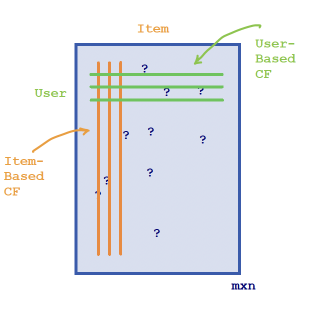
There are two types of collaborative filtering:
User-based CF: “Similar users will like similar items.” For example, if User A liked an item and User B has a similar profile to User A, it is likely that User B will also like that item. The challenge is defining what makes users similar.
Item-based CF: “Users will like items similar to those they have already liked.” For example, if User A liked Item X, and Item Y is similar to Item X, then User A is likely to like Item Y as well.
User-based Collaborative Filtering
The challenge in user-based collaborative filtering is to quantify resemblance between users (or, later, items) even when most ratings are missing. This means that we need a notion of similarity. Some of the most commonly used similarity metrics include:
Jaccard Similarity: compares users based on the items they have both interacted with, or compares items based on shared users. It is ideal for binary data. For explicit ratings one first binarizes (for example, “rated” versus “not rated”, or “liked” versus “not liked”): \[\frac{|A\cap B|}{|A\cup B|}, \quad \text{where } A, B \text{ are two sets.}\]
Cosine Similarity: measures the cosine of the angle between two vectors. Missing values are ignored, or equivalently treated as zeros: \[\frac{u^{\top} v}{\|u\| \cdot \|v\|}, \quad \text{where } u,v \text{ are two vectors.}\]
Centered Cosine Similarity (Pearson Correlation): A variation of cosine similarity that first subtracts a user’s (or item’s) mean rating: \[\frac{(u-\bar{u})^{\top} (v-\bar{v})}{\|u-\bar{u}\| \cdot \|v-\bar{v}\|}, \quad \text{where } u,v \text{ are two vectors.}\]
Cosine and Pearson coefficients fall in the range \([-1, 1]\), whereas a similarity used as a weight is often expected to lie in \([0, 1]\). Negative similarities are awkward in a weighted average, so in practice one either keeps only positive similarities or maps the coefficient to \([0,1]\) via \((1+\cos)/2\). In what follows we treat the similarity \(s_{au}\) as a weight and assume that convention has already been chosen.
The measures are computed from the shared, non-missing elements between two entities. For users \(u\) and \(v\), the calculation uses only items that both users have rated. Consequently the effective length of the vector for \(u\) can change depending on whether we compare \(u\) with \(v_1\) or \(u\) with \(v_2\). A common pathology is that two users who have rated only one item in common receive similarity \(1\).
Two conventions for centering are in use, and they are not the same:
- Center on all of a user’s ratings, then take cosine on co-rated items. If user \(u\) has rated 20 movies and 5 of those are also rated by user \(v\), the mean \(\bar{u}\) is computed from all 20 ratings, while the cosine uses only the 5 shared ratings. This is the usual implementation of Pearson correlation in recommender systems.
- Restrict everything, including the means, to co-rated items. In the same example, both the centering and the cosine use only the 5 shared ratings.
The displayed formula above corresponds to the second convention if \(\bar{u}\) and \(\bar{v}\) are computed on the co-rated support only. Finally, the denominator can become zero when all non-missing entries of a (centered) vector are constant, so those pairs must be skipped or regularized.
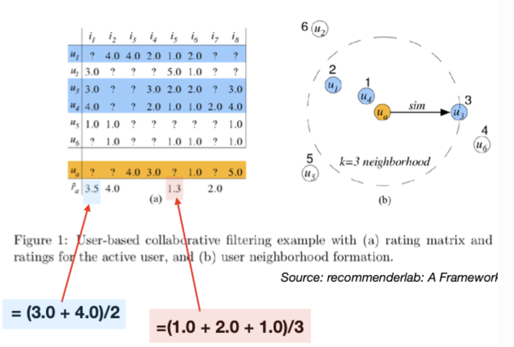
In the illustration above we used simple averages. We can extend this to weighted averages, using weights based on proximity to the user of interest. Let \(N(a)\) be the set of \(k\) nearest neighbors of user \(a\). The predicted rating of user \(a\) for item \(i\) is
\[ \hat{r}_{ai} = \frac{ \sum_{u \in N(a):\, r_{ui} \neq ?} s_{au}\, r_{ui} }{ \sum_{u \in N(a):\, r_{ui} \neq ?} s_{au} }. \]
The prediction is undefined if no neighbor of \(a\) has rated item \(i\). In practice, to reduce that problem, we select the nearest neighbors among users who have rated the item in question. The neighborhood of \(a\) may therefore change with \(i\). A mean-centered variant replaces \(r_{ui}\) by \(r_{ui}-\bar{r}_u\) and then adds \(\bar{r}_a\) back after the weighted average.
Item-Based Collaborative Filtering
In item-based collaborative filtering, we consider similarities between items instead of users. Below, a similarity matrix for items is constructed.
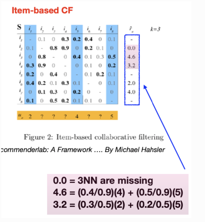
The top three entries in each row are highlighted in bold, since we consider only 3-nearest neighbors. For a test user, represented in orange, who has provided ratings for items 1, 5, and 8, these respective columns are highlighted in blue. These are the items the test user has rated, and their ratings will serve as the foundation for our predictions.
For the test user in question, the aim is to predict the ratings for the unreviewed items using the known ratings for items 1, 5, and 8.
Let \(S(i)\) be the set of \(k\) nearest items to item \(i\) (in the figure, \(k=3\)). The predicted rating \(\hat{r}_{ai}\) for item \(i\) from user \(a\) is a weighted average of \(a\)’s ratings on those neighbors that \(a\) has actually rated, with weights given by item-item similarities \(s_{ij}\):
\[ \hat{r}_{ai} = \frac{ \sum_{j \in S(i):\, r_{aj} \neq ?} s_{ij}\, r_{aj} }{ \sum_{j \in S(i):\, r_{aj} \neq ?} s_{ij} }. \]
The prediction is missing if the set \(\{j \in S(i): r_{aj} \neq ?\}\) is empty, i.e., when none of the similar items have been rated by the user. As in the user-based case, we can choose the neighbors of \(i\) dynamically among items that user \(a\) has rated, so that the neighborhood used for \(\hat{r}_{ai}\) can depend on \(a\).
Pros and Cons of Collaborative Filtering
Collaborative filtering does not rely on pre-defined item features: user interactions become the features, so the system can recommend items outside the user’s usual content profile. It cannot start from day one, because it needs a build-up of user-item interaction data. New items with no interaction history cannot be recommended; this is the cold start problem (the same issue appears for brand-new users). There is also a risk of popularity bias, in which items that many people have already rated are recommended to everyone and personalization is weakened.
Item-Based vs User-Based Collaborative Filtering
The choice between user-based and item-based collaborative filtering often depends on the specific context and platform.
For instance, e-commerce sites and streaming services such as Amazon and Netflix have often found item-based CF more effective. Item similarities tend to be more stable over time than user similarities, and “users who liked this also liked that” is a more reliable relation than the less predictable notion of similar people.
Neither algorithm is cheap if one identifies nearest neighbors by a brute-force scan of a large catalog. Approximation algorithms, clustering, and efficient data structures are used to keep the cost manageable.
Item-based CF also has a computational advantage in production. Both methods must find nearest neighbors, but item-based CF can push most of the work into an offline training phase: one builds and sorts an item-to-item similarity matrix once, then serves predictions from it. User-based CF has no comparable static training phase; similarities between users are computed at prediction time, which is expensive in real time.
The tradeoff is memory. The precomputed item-item matrix must be stored and accessed efficiently when recommendations are generated. If the catalog is huge one typically keeps only the top-\(k\) similarities per item.