11.4 Latent Factor Model
The latent factor model is another way to work with the rating matrix. The idea is inspired by a truncated singular value decomposition (SVD): we approximate the \(m \times n\) rating matrix by a product of two thinner factor matrices that embed users and items in a shared \(d\)-dimensional space.
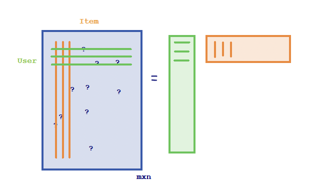
The decomposition is \[ R_{m \times n} \approx U_{m \times d}\, V^{\top}_{d \times n}, \] where \(V\) is \(n \times d\). The \(d\) columns of \(U\) are user factors and the \(d\) columns of \(V\) (equivalently, the \(d\) rows of \(V^{\top}\)) are item factors. A user’s predicted preference for an item is the inner product of the corresponding factor vectors. In a full SVD one would also have a diagonal matrix of singular values; here those scales are absorbed into \(U\) and \(V\).
Classical SVD cannot be applied directly, because \(R\) has missing entries. Instead we minimize a quadratic loss only over observed ratings. If every entry were observed, that minimizer would recover (a truncation of) the ordinary SVD. To avoid overfitting we add penalty terms on the factors. The resulting objective is
\[ \sum_{R_{ij} \neq ?} \bigl(R_{ij} - u_i^{\top} v_j\bigr)^2 + \lambda_1 \mathrm{Pen}(U) + \lambda_2 \mathrm{Pen}(V), \]
where \(u_i\), the \(i\)-th row of \(U\), is the latent vector for user \(i\), and \(v_j\), the \(j\)-th row of \(V\), is the latent vector for item \(j\). Typical penalties are squared Frobenius norms, \(\mathrm{Pen}(U)=\|U\|_F^2\) and \(\mathrm{Pen}(V)=\|V\|_F^2\).
This loss is convex in \(U\) for fixed \(V\) and convex in \(V\) for fixed \(U\), but it is not jointly convex in \((U,V)\). In practice one therefore uses alternating least squares (ALS), cycling between the two blocks, or stochastic gradient descent over observed ratings. After the factors have been fit, a missing entry is predicted by the inner product \(u_i^{\top} v_j\).
Taking this model further, we put the baseline from the previous section back in. The latent product is then asked only to explain what is left after \(\mu + a_i + b_j\):
\[ R_{ij} = \underbrace{\mu}_{\text{Overall Average} } + \underbrace{a_i}_{\text{User Effect}} + \underbrace{b_j}_{\text{Item Effect}} + u_i^{\top} v_j. \]
Substituting that into the loss, and regularizing \(a\) and \(b\) as well, gives
\[ \sum_{R_{ij} \neq ?} \bigl(R_{ij} - \mu - a_i - b_j - u_i^{\top} v_j\bigr)^2 + \lambda\bigl(\|U\|_F^2 + \|V\|_F^2 + \|a\|_2^2 + \|b\|_2^2\bigr). \]
The same ALS or SGD procedures apply. In practice the baseline alone already does a lot; the factors are there to capture the leftover user–item interactions.