Chapter 10 Classification Trees & Ensemble Methods
In this section we revisit trees in a different context. In contrast to regression trees, the response is now a categorical variable taking values in a discrete set, \(Y\in \{1, 2, \ldots, K\}\). Given features \(X = (X_1, X_2, \ldots, X_p)\), the goal is to assign a new observation to one of the \(K\) classes.
Tree-based methods, as discussed earlier, are nonparametric procedures that recursively partition the feature space into hyper-rectangular regions and make a constant prediction in each region. Historically there are two main lines of tree algorithms: Classification and Regression Trees (CART; Breiman, Friedman, Olshen, and Stone, 1984) and the ID3/C4.5 family (Quinlan, 1986, 1993).
As an illustration we use the Titanic survival data, a staple example for classification. The version in the chunk below was downloaded from Kaggle here. We use passenger class, sex, age, number of siblings/spouses aboard, and number of parents/children aboard to predict whether a passenger survived. Pruning works in the same way as for regression trees.
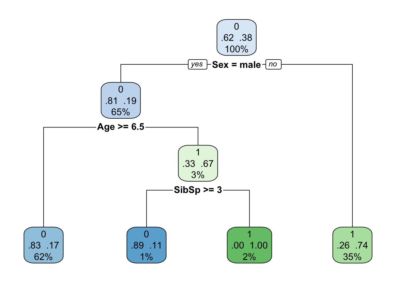
The terminal nodes show the idea of a classification tree: the algorithm recursively splits the feature space until each region is dominated by one class, and that majority class is the prediction for the region.
Once the tree is grown, the prediction in a terminal node \(\mathcal{T}\) is the majority class, \[ \hat{y}(x) = \arg\max_{k}\, \hat{p}_k\bigl(\mathcal{T}(x)\bigr), \] where \(\mathcal{T}(x)\) is the leaf that contains \(x\) and \(\hat{p}_k\) is the sample frequency of class \(k\) in that leaf. If a probability is needed later—for example to compare the tree with logistic regression—use \(\hat{p}_k\bigl(\mathcal{T}(x)\bigr)\) itself, not only the hard label.
The official Kaggle test file has no survival labels, so a fair comparison uses a holdout slice of the labeled training data. The table below reports misclassification for a majority-class baseline, the pruned tree, and a logistic regression on the same features.
set.seed(10)

# Complete cases so the tree and the logistic model see the
# same rows
titanic.cc = titanic.train[complete.cases(titanic.train[, c("Survived",
    "Pclass", "Sex", "Age", "SibSp", "Parch")]), ]
n.t = nrow(titanic.cc)
hold = sample(seq_len(n.t), size = floor(0.3 * n.t))
tr = titanic.cc[-hold, ]
te = titanic.cc[hold, ]

maj = as.numeric(names(which.max(table(tr$Survived))))
base.err = mean(te$Survived != maj)

tree.hold = rpart(as.factor(Survived) ~ Pclass + Sex + Age +
    SibSp + Parch, data = tr)
tree.hold = prune(tree.hold, cp = 0.02)
tree.err.tr = mean(predict(tree.hold, tr, type = "class") !=
    factor(tr$Survived))
tree.err.te = mean(predict(tree.hold, te, type = "class") !=
    factor(te$Survived))

glm.hold = glm(Survived ~ Pclass + Sex + Age + SibSp + Parch,
    data = tr, family = binomial())
glm.hat = as.integer(predict(glm.hold, te, type = "response") >
    0.5)
glm.err.te = mean(glm.hat != te$Survived)

data.frame(method = c("Majority class (holdout)", "Pruned tree (train)",
    "Pruned tree (holdout)", "Logistic regression (holdout)"),
    misclassification = round(c(base.err, tree.err.tr, tree.err.te,
        glm.err.te), 3))
## method misclassification
## 1 Majority class (holdout) 0.453
## 2 Pruned tree (train) 0.158
## 3 Pruned tree (holdout) 0.201
## 4 Logistic regression (holdout) 0.192A single tree is already better than the base rate. Whether it beats the logistic model depends on the split and on how nonlinear the signal is; the point of the table is to put the tree on the same scoreboard as the methods from the previous chapters, not to declare a winner.
The classification methods we have already discussed either transform the feature space (SVMs) or rely on a distance (\(k\)NN, kernel methods). A tree attacks the same problem by cutting the feature space directly into rectangles, using a binary splitting rule of the form \(\mathbf{1}_{\{x \leq c\}}\).