4.2 Splines Regression
Splines are piecewise polynomials thar are constructed so that thay can be both sensitive and smooth, but also capture local features of the data.
A Cubic Spline is a curve constructed from sections of cubic polynomials, joined together so that the curve is continuous up to second derivative. The points at which the sections join are called the knots of the spline. For a conventional spline, the knots occur wherever there is a datum, but for the regression splines the locations of the knots must be chosen. Typically, the knots would either be evenly spaced through the range of observed \(x\) values, or placed at the quantiles of the distribution of unique \(x\) values. Each section of cubic has different coefficients, but at the knots it will match its neighboring sections in value and first two derivatives.
Cubic Splines (Mathematical) Definition
A function \(g\) defined on \([a,b]\) is a cubic spline with respect to knots \(\{\xi_i\}_{i=1}^m\) (specifically \(a<\xi_1<\xi_2<\ldots<\xi_m<b\)) if:
\(g\) is a cubic polynomial in each of the \(m+1\) intervals, i.e. \[g(x) =d_ix^3+c_ix^2+b_ix+a_i,\quad x\in [\xi_i,\xi_{i+1}]\] where \(i=0,\ldots, m\), \(\xi_0=a\) and \(\xi_{m+1}=b\).
\(g\) is continuous up to the 2nd derivative. Since \(g\) is continuous up to the 2nd derivative for any point inside an interval, it suffices to check the following conditions: \[g^{(0,1,2)} (\xi_i^+)=g^{(0,1,2)}(\xi_i^-),\quad i=1, \ldots, m\] This expression indicates that the function and the first and second order derivatives are continuous at the knots.
How many free parameters do we need to represent a cubic spline?
(+) 4 parameters \((d_i,c_i,b_i,a_i)\) for each of the \((m+1)\) intervals.
(-) 3 constraints at each of the \(m\) knots (continuity constraints).
The total number of free parameters (similar to the number of degrees of freedom) is: \[4(m+1) - 3m = m + 4\]
A property of the cubic splines
Suppose the knots \(\{\xi_i\}_{i=1}^m\) are given.
- If \(g_1(x)\) and \(g_2(x)\) are cubic splines, the linear combination \[a_1g_1(x)+a_2g_2(x)\] is also a cubic spline, where \(a_1\) and \(a_2\) are known constants.
That is, for a set of given knots, the corresponding cubic splines form a linear space (of functions) with dim \((m + 4)\).
4.2.1 Examples of Cubic Splines Basis
- A set of basis functions for cubic splines (w.r.t knots \(\{\xi_i\}_{i=1}^m\)) is given by: \[\begin{align*} h_0(x)&= 1\\ h_1(x)&=x\\ h_2(x)&=x^2\\ h_3(x)&=x^3;\\ h_{i+3}(x) &= (x-\xi_i)_+^3,\quad i=1,2,\ldots,m\\ \end{align*}\] That is, any cubic spline can be uniquely expressed as: \[ \beta_0 +\sum_{j=1}^{m+3}\beta_j h_j(x)\]
- Given knot locations, there are many alternative, but equivalent ways of writing down a basis for cubic splines. For example, another basis for cubic splines can be written as: \[\begin{align*} h_0(x) &= 1\\ h_1(x) &= x\\ h_{i+1}(x) &= R(x, \xi_i^*),\,\, i=1, \ldots, q-1 \end{align*}\] where \[\begin{align*} R(x,z) &= \left[ (z-1/2)^2 - 1/12\right] \left[ (x-1/2)^2 - 1/12\right]/4\\ & \quad \,- \left[ (|x-z|-1/2)^4 - 1/2 (|x-z|-1/2)^2 + 7/240\right] /24\\ \end{align*}\]
An Example of a Cubic Splines Basis
We first define the function \(R(x,z)\) as above in R:
R_xz <- function(x, z) {
    ((z - 0.5)^2 - 1/12) * ((x - 0.5)^2 - 1/12)/4 - ((abs(x -
        z) - 0.5)^4 - (abs(x - z) - 0.5)^2/2 + 7/240)/24
}
We then need to define the knots
In regression examples the \(x\) variable will be the predictor (there is no need to generate any \(x\) values). Here, we need a “generic” \(x\) for illustration purposes.
Finally, we defined the splines functions, based on the definition given above:
spline1 = rep(1, length(x))  # First basis function
spline2 = x  # Second basis function
spline3 = R_xz(x, new.knots[1])  # Third basis function
spline4 = R_xz(x, new.knots[2])  # Fourth basis function
spline5 = R_xz(x, new.knots[3])  # Fifth basis function
If we want to represent a function using the basis above, we have:
For illustration purposes, we plot the basis functions defined above as well as the function \(f\):
par(mfrow = c(2, 3))
plot(x, spline1, type = "l", lty = 3, ylab = expression("h"[0] *
    "(x)=1"))
plot(x, spline2, type = "l", lty = 3, ylab = expression("h"[1] *
    "(x)=x"))
plot(x, spline3, type = "l", lty = 3, ylab = expression(paste(h[2](x)) *
    "=" * paste(R(x, xi[1]))))
plot(x, spline4, type = "l", lty = 3, ylab = expression(paste(h[3](x)) *
    "=" * paste(R(x, xi[2]))))
plot(x, spline5, type = "l", lty = 3, ylab = expression(paste(h[4](x)) *
    "=" * paste(R(x, xi[3]))))
plot(x, fun1s, type = "l", ylab = "f(x)", main = expression("f(x) =  4 - 0.05 h"[1] *
    " - 6 h"[2] * "+ 2 h"[3] * "+ 10 h"[4]), col = "blue", lwd = 2)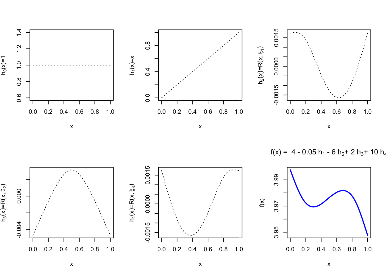
4.2.2 B-Splines Basis Functions in R
In this course one of the cubic spline bases we will use is the B-spline basis.
Cubic B Splines Definition
The cubic B-spline basis on an interval $ [a,b] $ with interior knots $ {i}{i=1}^m $ satisfies the following properties:
Each basis function is nonzero only on an interval spanned by four successive knots (and is zero elsewhere).
On every sub-interval between consecutive knots the basis function is a cubic polynomial.
The basis function is continuous and has continuous first and second derivatives at every knot.
The basis function integrates to 1 over its support.
The two boundary basis functions are modified so that the required continuity conditions hold at the endpoints \(a\) and \(b\).
These bases are provided by the splines library in R; the generating function is bs().
Its main arguments are
x: the predictor vector.df: desired degrees of freedom (number of columns of the returned basis matrix).knots: vector of interior knot locations.degree: degree of the piecewise polynomial (default = 3, i.e., cubic).intercept: ifTRUEan intercept column is included in the basis; default isFALSE.(This is not the intercept of the eventual regression model.)Boundary.knots: the two boundary knots at which the basis is anchored; by default they are set to the range of the non-missing values ofx
(The full documentation is available here.)
In practice we supply either the vector knots or the integer df, but not both. All other arguments are left at their defaults.
The value returned by bs() is a matrix with length(x) rows.
If df is supplied the matrix has df columns.
If knots is supplied the number of columns equals \[\text{length(knots)} + \text{degree} + \text{as.integer(intercept)}.\] With the default
intercept = FALSEthis reduces to length(knots) + 3.
Specifying knots versus degrees of freedom**
If the knot locations are known, pass them via the knots argument:
Defining knots location in bs()
library(splines)
x = seq(0, 1, by = 0.01)  # generic `x` for illustration purposes
new.knots = c(1/6, 3/6, 5/6)  # define three knots at locations 1/6, 3/6, 5/6.
Bsplines.basis1 = bs(x, knots = new.knots)
head(Bsplines.basis1)
## 1 2 3 4 5 6
## [1,] 0.000000 0.0000000 0.0000000 0 0 0
## [2,] 0.165912 0.0034896 0.0000144 0 0 0
## [3,] 0.304896 0.0135168 0.0001152 0 0 0
## [4,] 0.418824 0.0294192 0.0003888 0 0 0
## [5,] 0.509568 0.0505344 0.0009216 0 0 0
## [6,] 0.579000 0.0762000 0.0018000 0 0 0In this case, R sets
\[\text{df = length(knots) + degree}\]
(or one more if if intercept=TRUE).
- If a target degrees of freedom is preferred, pass
df. Thenbs()places df - degree interior knots at suitable quantiles ofx(ordf - degree - 1knots whenintercept = TRUE).
Specifying degrees of freedom with bs()
x = seq(0, 1, by = 0.01)  # generic `x` for illustration purposes
Bsplines.basis2 = bs(x, df = 4)
head(Bsplines.basis2)
## 1 2 3 4
## [1,] 0.000000 0.000000 0.000000 0
## [2,] 0.058214 0.000592 0.000002 0
## [3,] 0.112912 0.002336 0.000016 0
## [4,] 0.164178 0.005184 0.000054 0
## [5,] 0.212096 0.009088 0.000128 0
## [6,] 0.256750 0.014000 0.000250 0
The following code illustrates the first six B-spline basis functions obtained from the three knots defined above.
Illustration of B Splines Basis Function
## [1] 101 6## 1 2 3 4 5 6
## [1,] 0.000000 0.0000000 0.0000000 0 0 0
## [2,] 0.165912 0.0034896 0.0000144 0 0 0
## [3,] 0.304896 0.0135168 0.0001152 0 0 0
## [4,] 0.418824 0.0294192 0.0003888 0 0 0
## [5,] 0.509568 0.0505344 0.0009216 0 0 0
## [6,] 0.579000 0.0762000 0.0018000 0 0 0par(mfrow = c(2, 3))
plot(x, Bsplines.basis[, 1], type = "l", lty = 3, ylab = expression(paste(h[1](x))))
plot(x, Bsplines.basis[, 2], type = "l", lty = 3, ylab = expression(paste(h[2](x))))
plot(x, Bsplines.basis[, 3], type = "l", lty = 3, ylab = expression(paste(h[3](x))))
plot(x, Bsplines.basis[, 4], type = "l", lty = 3, ylab = expression(paste(h[4](x))))
plot(x, Bsplines.basis[, 5], type = "l", lty = 3, ylab = expression(paste(h[5](x))))
plot(x, Bsplines.basis[, 6], type = "l", lty = 3, ylab = expression(paste(h[6](x))))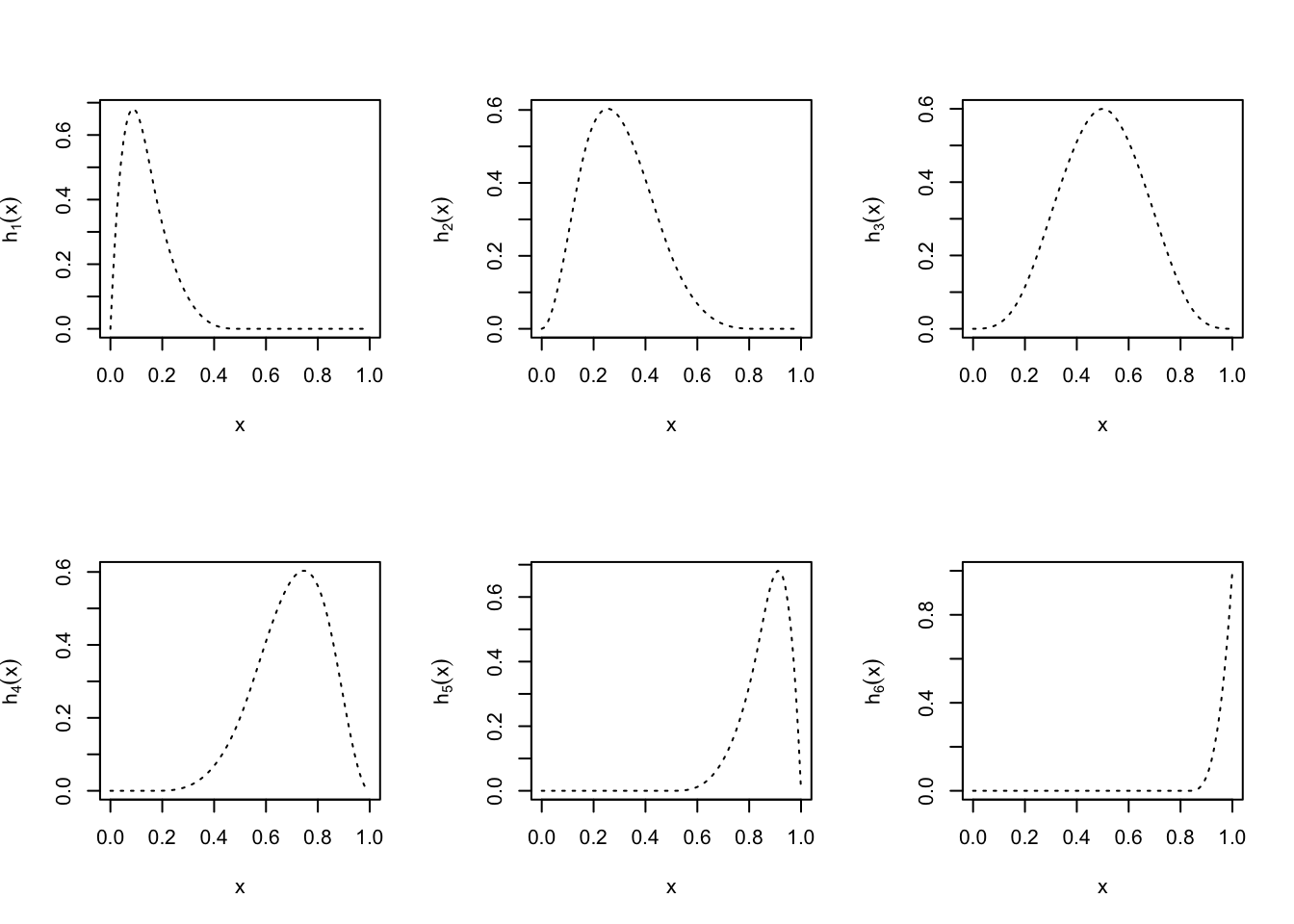
4.2.3 Natural Cubic Splines (NCS)
A cubic spline on \([a,b]\) is called a natural cubic spline if its second and third derivatives vanish at the endpoints \(a\) and \(b\). Consequently the spline is linear on the two extreme intervals \([a,\xi_1]\) and \([\xi_m,b]\). The linearity constraints reduce the dimension of the space: a natural cubic spline with \(m\) interior knots has only \(m\) degrees of freedom (the usual textbook count).
Remark
If we place a knot at every distinct observation \[ x_i \] and use a natural cubic spline, the resulting interpolant is a smooth curve that passes through every data point \[ (x_i,y_i) \].
Natural Cubic Spline
One convenient basis for the space of natural cubic splines with \(m\) interior knots is \[\begin{align*} N_1(x) &= 1\\ N_2(x) &= x\\ N_{k+2} (x) &= d_k(x) - d_{k-1}(x) \end{align*}\] where \[d_k(x) = \frac{(x-\xi_k)_{+}^{3} - (x-\xi_{m})_{+}^{3}}{\xi_m - \xi_k}\] Each of these functions has vanishing second and third derivatives for \(x\ge\xi_m\).
In R natural cubic splines are generated by the function ns() from the same splines package:
\[ ns(x, df, knots, intercept=FALSE, Boundary.knots) \] (Note that the default value of intercept is FALSE, exactly as for bs().)
Natural Cubic Splines in R
## [1] 101 4par(mfrow = c(2, 3))
plot(x, NCS.basis[, 1], type = "l", lty = 3, ylab = expression(paste(h[1](x))))
plot(x, NCS.basis[, 2], type = "l", lty = 3, ylab = expression(paste(h[2](x))))
plot(x, NCS.basis[, 3], type = "l", lty = 3, ylab = expression(paste(h[3](x))))
plot(x, NCS.basis[, 4], type = "l", lty = 3, ylab = expression(paste(h[4](x))))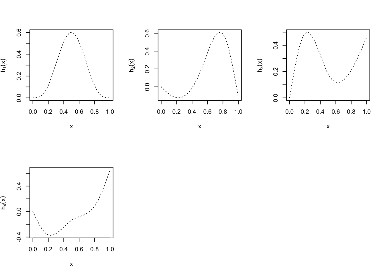
Because the spline is forced to be linear outside the boundary knots, observations that fall outside those knots do not influence the fit. By default, therefore, R places the boundary knots at the minimum and maximum of the observed \[ x_i \].
Knots versus degrees of freedom for ns()
If interior knot locations are supplied, the number of columns of the basis matrix is
\[ \text{length(knots)} + 1 + \text{as.integer(intercept)}\]If a target
dfis supplied, R places
\[ m = \text{df} - 1 - \text{intercept}\] interior knots at quantiles of \(x\).
4.2.4 Regression Splines
For a fixed set of knots the corresponding cubic splines form a linear space of dimension \[ m+4 \]. Regression splines simply expand the mean function in this basis:
\[g(x)=\beta_1 h_1(x)+\beta_2 h_2(x)+\ldots+\beta_p h_p(x)\]
Ordinary Cubic Splines: \(p=m+4\).
Natural Cubic Splines (NCS): \(p=m\).
On the observed data the model may be written in matrix form \[ \begin{pmatrix} y_1\\ y_2\\ \ldots\\ y_n \end{pmatrix}_{n\times 1} = \begin{pmatrix} h_1(x_1)& \ldots & h_{p}(x_1)\\ h_1(x_2)& \ldots & h_{p}(x_2)\\ \\ h_1(x_n)& \ldots & h_{p}(x_n) \end{pmatrix}_{n\times p} \begin{pmatrix} \beta_1\\ \beta_2\\ \ldots\\ \beta_p \end{pmatrix}_{p\times 1} \] where the $ np$ matrix \(\mathbf{F}\) contains the basis functions evaluated at the \(x_i\). The coefficient vector is obtained by ordinary least squares: Therefore, we can estimate the coefficients \(\mathbf{\beta}\) by solving the following Least-Squares problem: \[\hat{\mathbf{\beta}}= \arg\min_{\mathbf{\beta}}||\mathbf{y} - \mathbf{F}{\mathbf{\beta}|}|^2\]
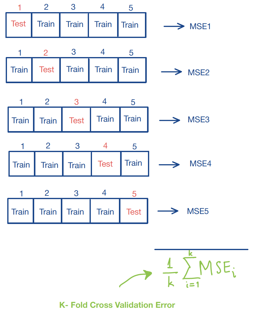
4.2.5 K-Fold Cross-Validation
A practical difficulty with regression splines is the choice of the number (and location) of knots, or equivalently the degrees of freedom. One systematic approach is \[ K \]-fold cross-validation:
Fix a candidate number of knots (or degrees of freedom).
Randomly partition the data into \(K\) roughly equal folds.
For each fold \(k=1,\dots,K\):
hold fold \(k\) out as a validation set,
fit the regression spline on the remaining \(K-1\) folds,
compute the mean squared error \(\mathrm{MSE}_k\) on the held-out fold.
Average the \(K\) errors: \[\mathrm{CV}(K) = \frac1K\sum_{k=1}^K\mathrm{MSE}_k.\]
Repeat the whole procedure for every candidate number of knots / degrees of freedom.
Select the value that minimises \(\mathrm{CV}(K)\).
A schematic illustration of the procedure appears below.