8.2 Logistic Regression with Separable Data
Consider the following scenario with two classes, each containing two points. Assume that the intercept is zero for simplicity.
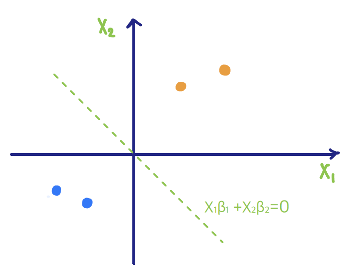
In the log-likelihood, the contribution of the orange points (\(y=1\)) involves \[\frac{e^{\beta_1 x_1 + \beta_2 x_2}}{1 + e^{\beta_1 x_1 + \beta_2 x_2}} = \frac{1}{1+ e^{-(\beta_1 x_1 + \beta_2 x_2)}},\] while the contribution of the blue points (\(y=0\)) involves \[\frac{1}{1 + e^{\beta_1 x_1 + \beta_2 x_2}}.\] The only difference between the two expressions is a minus sign in the exponent.
In this setting, as the \(\beta\)s grow in a separating direction, the fitted probabilities approach \(0\) or \(1\) and the likelihood keeps increasing, so the algorithm does not converge. The decision boundary itself stays the same, so the fitted classifier can still be used for prediction.
Remark: A natural question is whether regularization helps. An \(L_2\) (ridge) penalty with \(\lambda>0\), and typically an \(L_1\) (lasso) penalty as well, keeps the coefficients finite. The unpenalized MLE is the quantity that diverges: when the classes are perfectly separable, the likelihood increases as \(\|\beta\|\to\infty\) along a separating direction, and \((\beta_0,\beta)\) is no longer a well-defined interior maximizer.