12.5 Spectral Clustering
In some applications, we do not have the value of each data point, instead, we have the similarities between data points. Note that for similarity measures, larger means more similar, while for distance measures, larger is further away. A way to represent the data is the Similarity Graph \(G = (V,E)\) (an undirected graph) in which \(V\) is a set of vertices \(\{x_1, x_2, \ldots, x_n \}\), and \(E\) is the set of edges \(\{(i,j)\}_{ij}\).
For our case, this graph is weighted by an adjacency matrix \[\mathbf{W}_{n \times n} = \{w_{ij}\}_{ij}\]
We can define \(\mathbf{W}\) in many different ways. Each \(w_{ij}\) is the similarity between vertices \(i\) and \(j\) which means that \(\mathbf{W}\) is symmetric \(w_{ij} = w_{ji}\).
We also define the degree matrix \(D\) as a diagonal matrix \[diag(d_1, \ldots, d_n)\] where \(d_i\) is the degree of vertex \(i\): \[d_i = \sum_{j=1}^{n} w_{ij}\]
Graph Laplacian
There are many different ways to define a graph Laplacian matrix:
Unnormalized graph Laplacian: \[\mathbf{L} = \mathbf{D} - \mathbf{W}\]
Normalized graph Laplacians:
\[\begin{align*} \mathbf{L}_{sym} &= \mathbf{D}^{-1/2} \mathbf{L} \mathbf{D} ^{-1/2} = \mathbf{I} - \mathbf{D}^{-1/2} \mathbf{W} \mathbf{D}^{-1/2}\\ \mathbf{L}_{rw} &= \mathbf{D}^{-1} \mathbf{L} = \mathbf{I} - \mathbf{D}^{-1}\mathbf{W}\\ \end{align*}\]
Each of them has some unique properties:
For the unnormalized graph Laplacian, we have, for any \(f\)
\[\begin{align*}
f'\mathbf{L} f &= f'\mathbf{D} f - f'\mathbf{W} f = \sum_{i=1}^{n} d_i f_i^2 - \sum_{ij} f_i f_j w_{ij}\\
&= \frac{1}{2} \Biggl\{ \sum_{i} d_i f_i^2 - 2\sum_{i,j} f_i f_j w_{ij} + \sum_j d_j f_j^2 \Biggr\}\\
&= \frac{1}{2} \sum_{i,j} w_{ij} (f_i - f_j)^2
\end{align*}\]
\(L\) here is positive semi-definite. The smallest eigen-value is 0, with eigen-vector 1. The number of 0 eigen-values depends on the number of connected components.
For the normalized graph Laplacian, we have \[f' \mathbf{L}_{sym} f = \frac{1}{2} \sum_{i,j} w_{ij} \Bigl( \frac{f_i}{\sqrt{d_i}} - \frac{f_j}{\sqrt{d_j}} \Bigr)^2\] The eigenvalue \(\lambda\) and eigenvector \(\mathbf{v}\) of \(\mathbf{L}_{rw}\) can be solved from \[\mathbf{L}\mathbf{v} = \lambda \mathbf{D}\mathbf{v}\] The smallest eigenvalue of both \(\mathbf{L}_{sym}\) and \(\mathbf{L}_{rw}\) are 0, with eigenvectors \(\mathbf{1}\) and \(\mathbf{D}^{1/2}\mathbf{1}\) respectively.
The spectral clustering is very simple:
Clustering Algorithm
Construct a weighted adjacency matrix \(\mathbf{W}\), using e.g., \[w_{ij} = \exp \Biggl( -\frac{1}{2\sigma^2} ||x_i - x_j||^2\Biggr)\]
Compute the Laplacian \(\mathbf{L}\) (or normalized versions \(\mathbf{L}_{sym}\) and \(\mathbf{L}_{rw}\) )
Compute the smallest \(k\) eigenvectors, denote as \(\mathbf{V}_{n \times k}\). (For \(\mathbf{L}_{sym}\), a common extra step is to row-normalize \(\mathbf{V}\) before clustering.)
Treat \(\mathbf{V}_{n \times k}\) as the matrix of the observed data, and perform \(k\)-means clustering.
Output the \(k\) cluster labels
Below is an example from Von Luxburg, Ulrike. “A tutorial on spectral clustering.” Statistics and computing 17, no. 4 (2007): 395-416.
Spectral Clustering Example
Spectral clustering essentially consists of two steps. First, we construct the graph Laplacian \(\mathbf{L}\) (or normalized version), then we perform eigen-decomposition of the matrix. Let’s show an example, replicated from Von Luxburg (2007).
set.seed(1)
n = 50
x = c(rnorm(n, 0, 0.2), rnorm(n, 2, 0.2), rnorm(n, 4, 0.2), rnorm(n,
    6, 0.2))
hist(x, breaks = 100)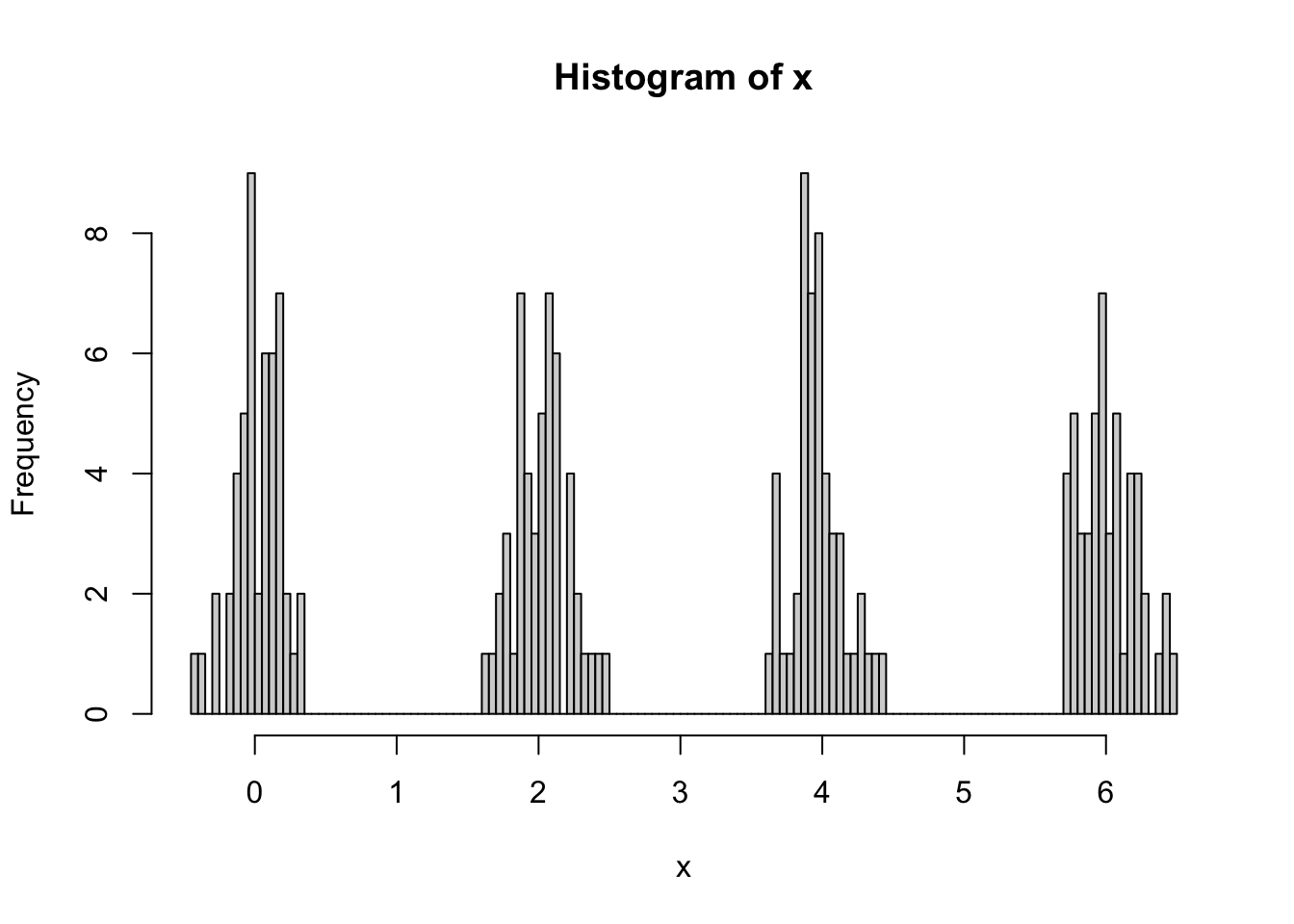
We use the adjacency matrix defined as \[w_{ij} = \exp\bigg\{\frac{- \lVert x_i - x_j\rVert^2 }{2 \sigma^2 } \bigg\},\] and calculate the Laplacian \[\mathbf{L} = \mathbf{D} - \mathbf{W}.\] We can then use the eigen decomposition to recover the underlying features.
# construct the adjacency matrix
W = as.matrix(exp(-dist(as.matrix(x))^2/4))
heatmap(W, Rowv = NA, Colv = NA, symm = TRUE, revC = TRUE)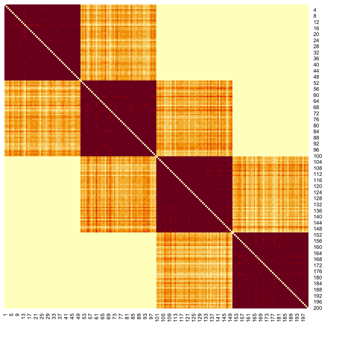
# compute the degree of each vertex
d = colSums(W)

# the laplacian matrix
L = diag(d) - W

# eigen decomposition
f = eigen(L, symmetric = TRUE)

# plot the eigen values we need the smallest ones
plot(rev(f$values)[1:20], pch = 19, ylab = "eigen-values", col = c(rep("red",
    4), rep("blue", 196)))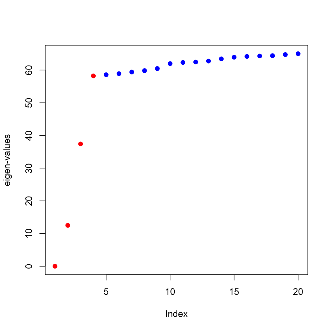
# plot the last four eigen vectors
par(mfrow = c(1, 4))
plot(f$vectors[, 200], type = "l", ylab = "eigenvector", ylim = c(-0.15,
    0.15))
plot(f$vectors[, 199], type = "l", ylab = "eigenvector", ylim = c(-0.15,
    0.15))
plot(f$vectors[, 198], type = "l", ylab = "eigenvector", ylim = c(-0.15,
    0.15))
plot(f$vectors[, 197], type = "l", ylab = "eigenvector", ylim = c(-0.15,
    0.15))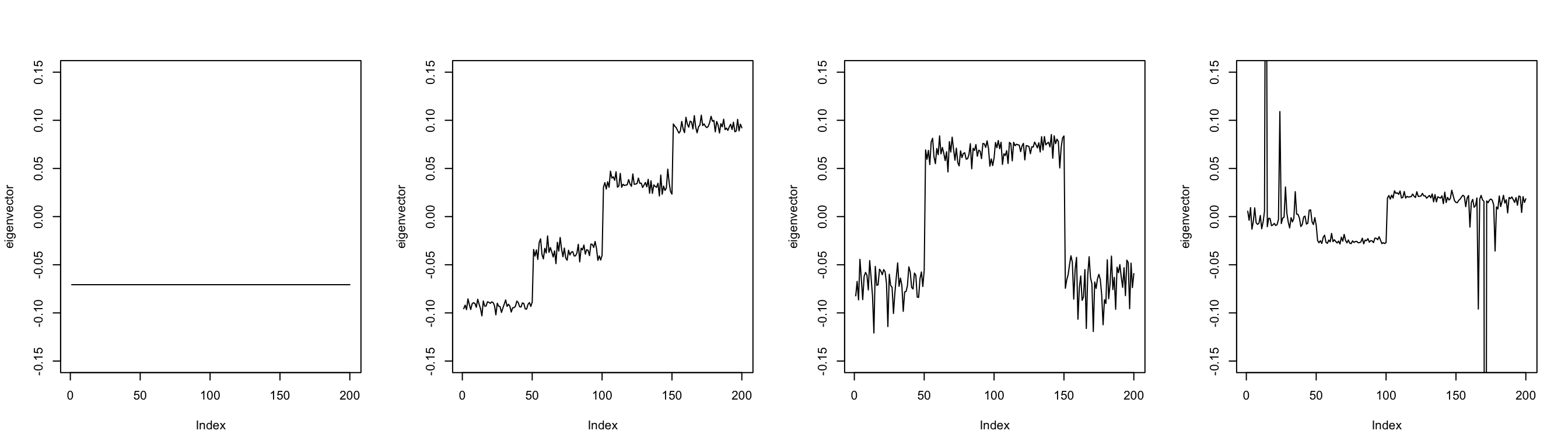
On the other hand, if we use an adjacency matrix that contains several non-connected blocks, then we would observe four zero eigen values. For example, using the KNN adjacency index, we may obtain four separated blocks.
##
## Attaching package: 'FNN'
## The following objects are masked from 'package:class':
##
## knn, knn.cvnn = get.knn(x, k = 10)
W = matrix(0, 200, 200)
for (i in 1:200) W[i, nn$nn.index[i, ]] = 1
# W is not necessarily symmetric
W = pmax(W, t(W))
heatmap(W, Rowv = NA, Colv = NA, symm = TRUE, revC = TRUE)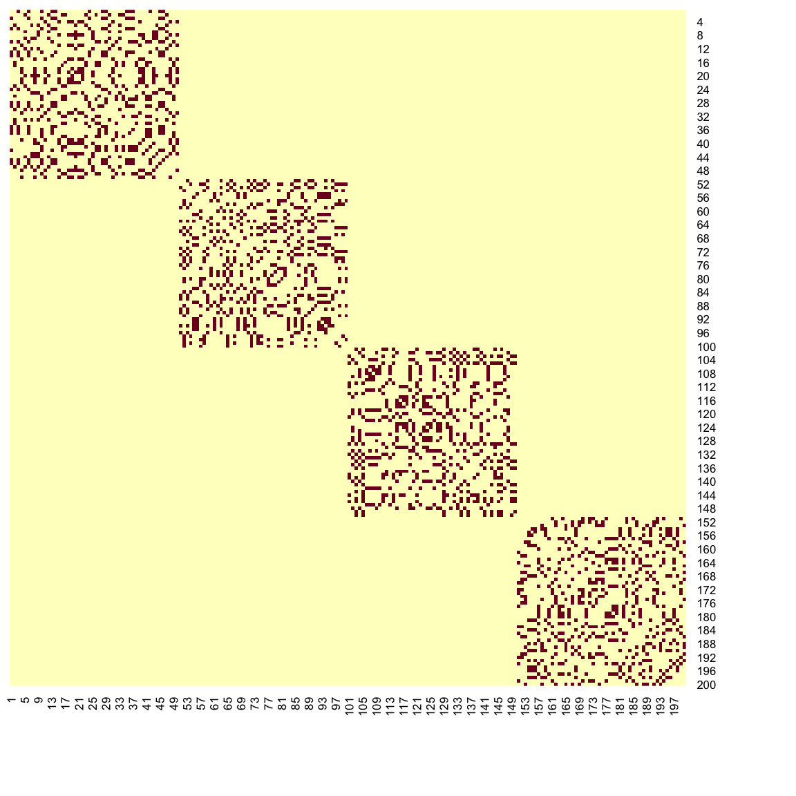
We use a normalized graph Laplacian, defined as \[\mathbf{L}_\text{sym} = \mathbf{I} - \mathbf{D}^{-1/2} \mathbf{W} \mathbf{D}^{-1/2}\]
# compute the degree of each vertex
d = colSums(W)

# the laplacian matrix
L = diag(200) - diag(1/sqrt(d)) %*% W %*% diag(1/sqrt(d))

# eigen decomposition
f = eigen(L, symmetric = TRUE)

# plot the eigen values we need the smallest ones
plot(rev(f$values)[1:20], pch = 19, ylab = "eigen-values", col = c(rep("red",
    4), rep("blue", 196)))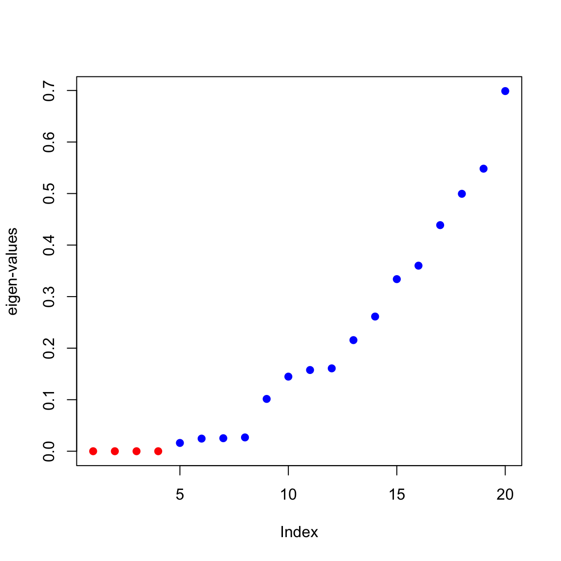
# plot the last four eigen vectors
par(mfrow = c(1, 4))
plot(f$vectors[, 200], type = "l", ylab = "eigenvector", ylim = c(-0.15,
    0.15))
plot(f$vectors[, 199], type = "l", ylab = "eigenvector", ylim = c(-0.15,
    0.15))
plot(f$vectors[, 198], type = "l", ylab = "eigenvector", ylim = c(-0.15,
    0.15))
plot(f$vectors[, 197], type = "l", ylab = "eigenvector", ylim = c(-0.15,
    0.15))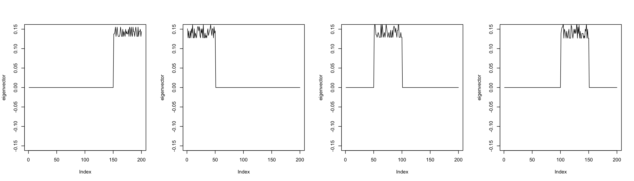
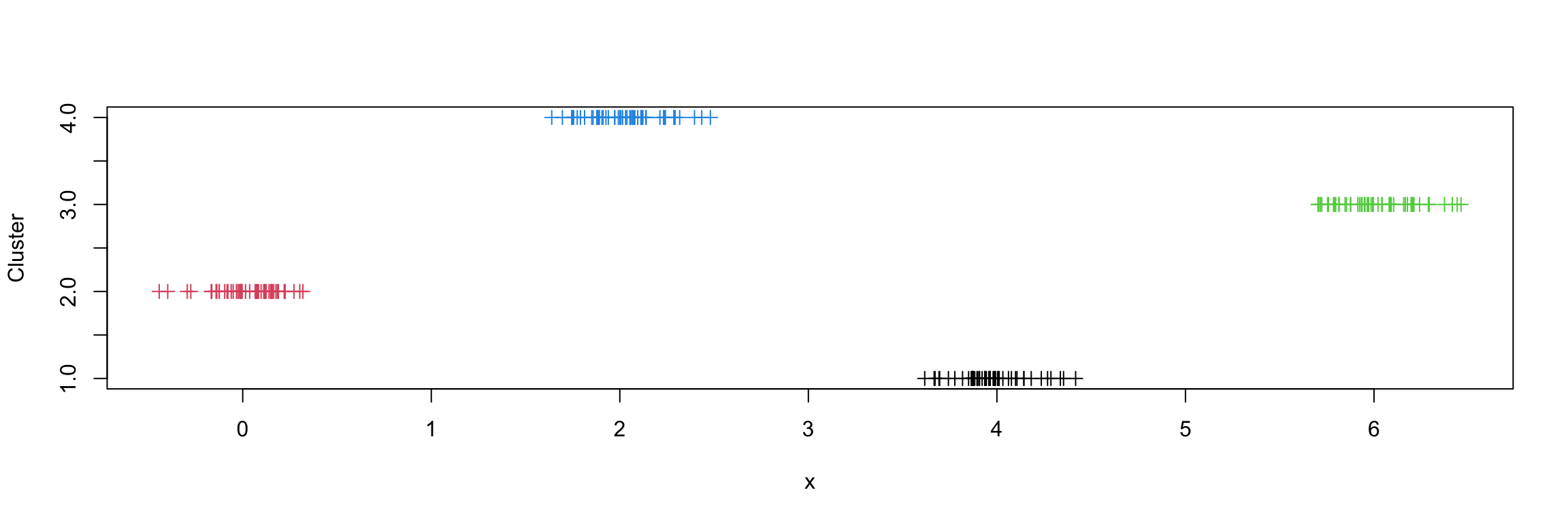
We can then perform \(k\)-means clustering using the top eigen vectors as the features.
cl = kmeans(f$vectors[, 197:200], centers = 4, nstart = 100)
plot(x, cl$cluster, ylab = "Cluster", col = cl$cluster, pch = 3)