Chapter 6 Regression Trees
In this section, we are going to discuss tree-based models for regression.
Framework
- Response Variable: \(Y\in \mathbb{R}\) – continuous
- Features: \(X = (X_1, X_2, \ldots, X_p)\)
Regression trees are non-linear and non-parametric methods. They recursively partition the feature space into hyper-rectangular subsets and fit a simple prediction in each piece. There is no single global form such as “\(Y\) is linear in \(X\)”; complexity is controlled by tuning parameters (tree size, and later the ensemble size). For this chapter both the split criterion and the leaf prediction use squared error. Classification trees (Gini, deviance) will wait.
Below we can see a sketch of a regression tree for awines data set in which we want to predict the quality of the wine (a numerical outcome) versus wine characteristics (a set of predictors):
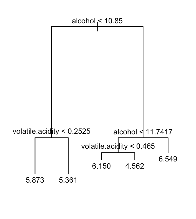
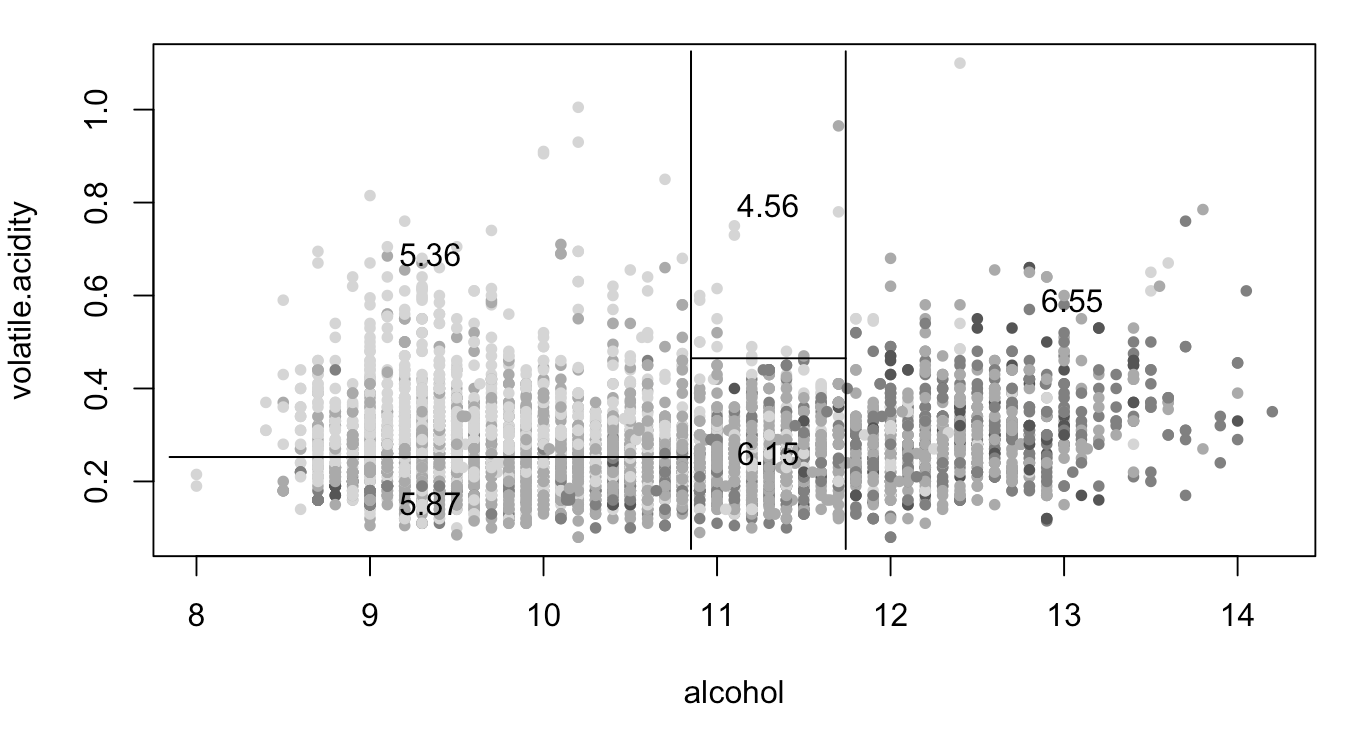
We will restrict our focus to binary partitions of the tree. In the example above, we first split the space into two regions and model the response by the mean of \(Y\) in each region. At each step, we choose the variable and split-point to achieve the best fit. Then one or both regions are split into two more regions, and this process continues until some stopping rule is applied. In the example, the first split is whether alcohol is less than or greater than \(10.85\). The region with \(\text{alcohol}<10.85\) is then split on volatile.acidity at \(0.2525\), and the region to the right is split on alcohol again at \(11.7417\), and so on. When we stop, the predicted quality is the average of \(Y\) in that region.
Terminology
- Leaf Node: Each leaf node corresponds to a rectangular-shaped region in the feature space.
- Internal Node: These nodes are parent nodes with two children – left and right nodes.
- A split involves a variable \(j\) and a particular split value \(s\).
A single tree is easy to interpret: a prediction is a short sequence of threshold rules. Splits depend only on the ordering of a predictor, so any monotone transformation of a predictor leaves the tree unchanged. The same splitting algorithm can be used when \(p\) is large, interactions appear when different variables are chosen along a path, and predictors that are never selected are effectively ignored.
The usual weakness is accuracy. One tree is often a high-variance fit; that is the reason for the ensemble methods later in this section.