12.4 Self-Organizing Maps
Self-organizing Map (SOM) is another popular clustering method. The main difference between SOM and \(K\)-means is that the cluster means of a SOM have a geometric relationship preserving the geometry of the underlying data. An SOM starts with Input Data: \(\{x_i\}_{i=1}^{n}\), with each \(x_i \in \mathbb{R}^{p}\). We then randomly initialize the Cluster Means, i.e. creating a grid of centers \(w_{ij} \in \mathbb{R}^{p}\), \(i=1, \ldots, q_1\), \(j=1,\ldots, q_2\). These are similar to the centers in a \(K\)-means algorithm, but they also preserve some geometric relationship on the grid. Then, we pick a Learning Rate: \(\alpha \in[0,1]\). This controls how fast the \(w_{ij}\)’s are updated, and it will decrease progressively. We also need to choose the Radius: \(r\). This controls how many \(w_{ij}\)’s will be updated at each iteration, and it will also decrease progressively.
SOM Algorithm
For \(k = 1, \ldots, n\), we will stream in one new observation \(x_k\) and perform the following update:
For all \(w_{ij}\), calculate the distance between each \(w_{ij}\) and \(x_k\). \ Let \(d_{ij} =\|x_k - w_{ij}\|\) (use Euclidean distance).
Select the closest \(w_{ij}\), denoted as \(w_{*}\).
Update each \(w_{ij}\) based on the formula \[w_{ij} \leftarrow w_{ij} + \alpha \, h(w_{*}, w_{ij}, r)\, (x_k - w_{ij})\] where \(h\) is a neighborhood function on the grid (typically depending on the grid distance between units and the current radius \(r\)). Units close to the winner on the map are pulled toward \(x_k\); units outside the neighborhood are left unchanged.
Decrease the value of \(\alpha\) and \(r\).
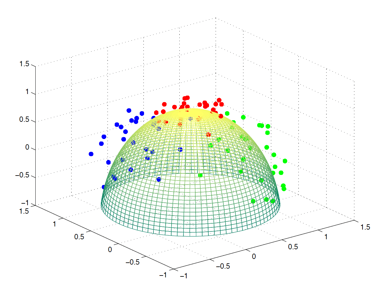
Figure 12.1: Self-Organizing Map (Ref. ESL textbook)
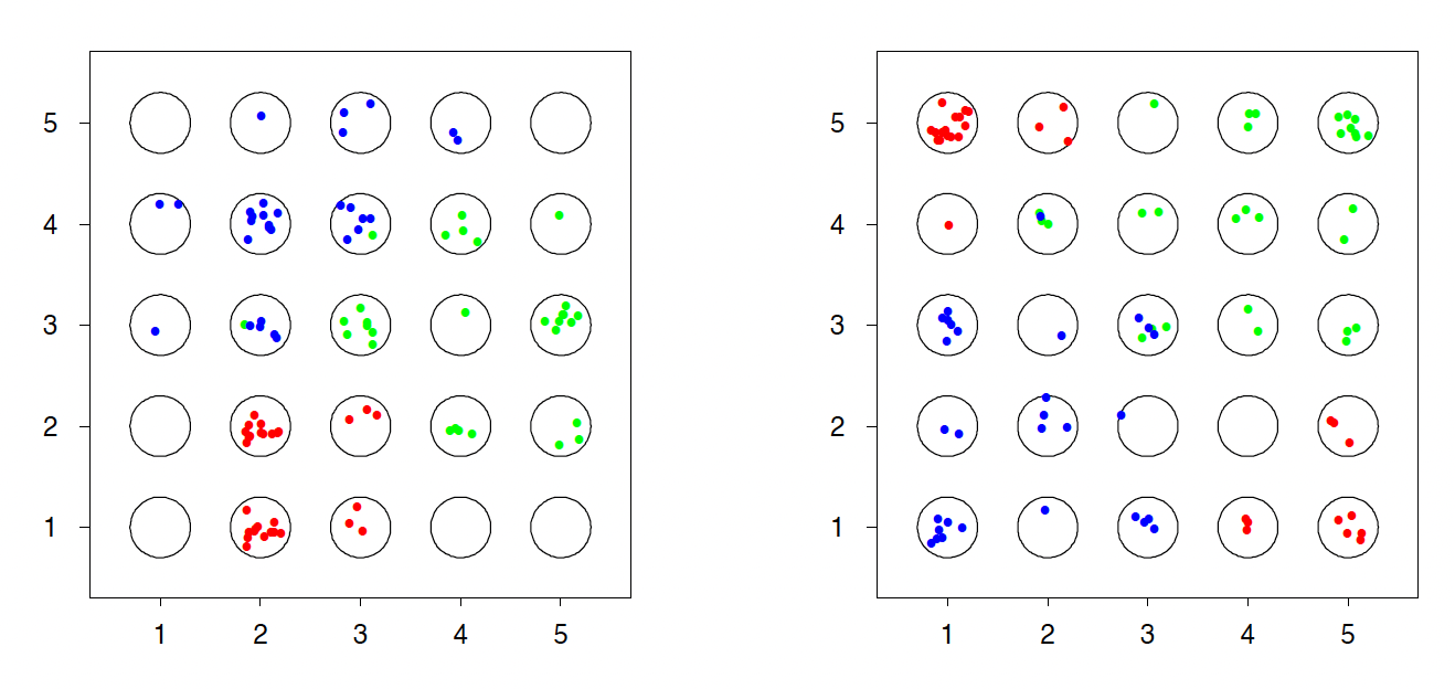
Figure 12.2: Self-Organizing Map (Ref. ESL textbook)
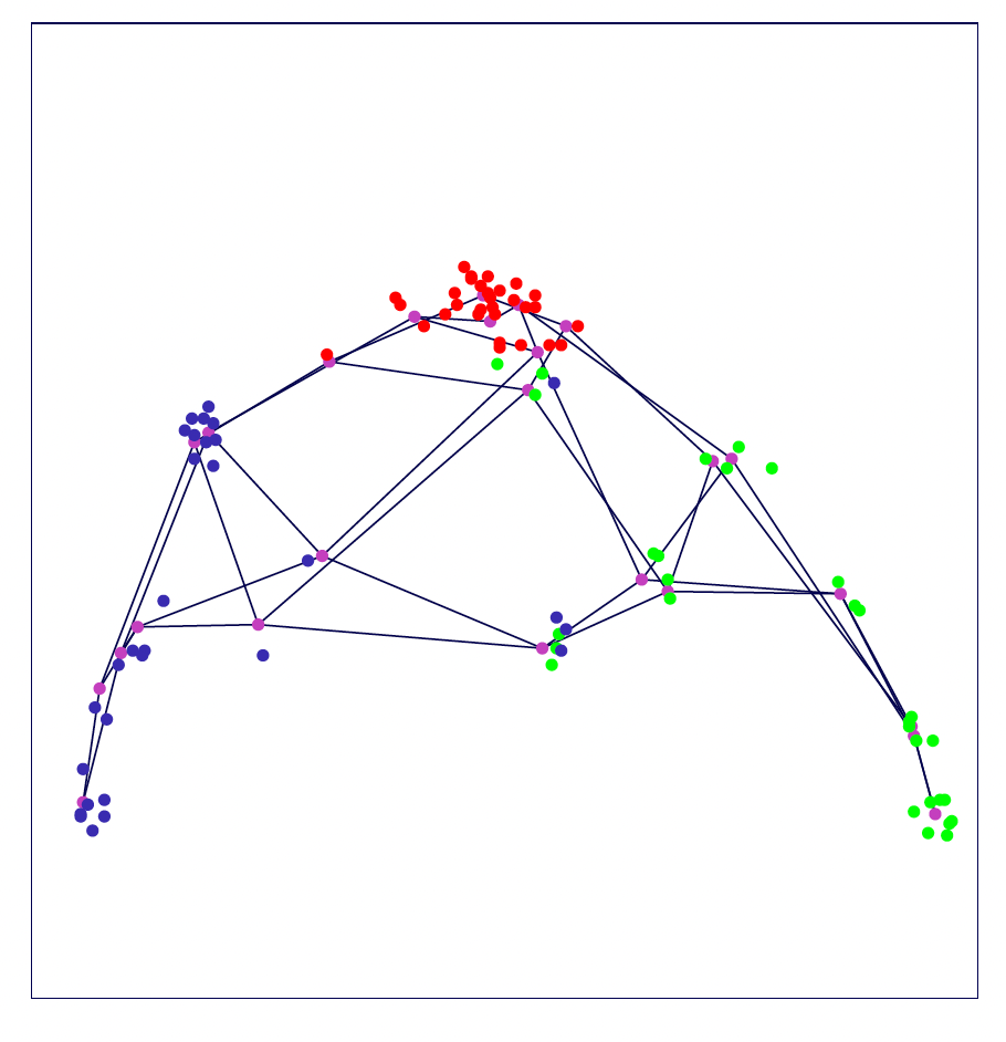
Figure 12.3: Self-Organizing Map (Ref. ESL textbook)