9.4 SVM as a Penalization Method
The soft-margin constraint \(y_i f(x_i)\ge 1-\xi_i\) with \(\xi_i\ge 0\) is equivalent to \(\xi_i\ge \bigl(1-y_i f(x_i)\bigr)_+\). Substituting the smallest feasible slacks into the primal objective gives \[ \operatorname{minimize}_{f}\ \sum_{i=1}^{n}\bigl(1-y_i f(x_i)\bigr)_+ + \lambda\|\beta\|^2, \] where \(\lambda=1/C\) and \(f(x)=x^T\beta+\beta_0\). This is a loss + penalty problem. The loss is the hinge loss \[ L(y,f(x))=\bigl(1-yf(x)\bigr)_+ = \max\bigl(0,\ 1-yf(x)\bigr). \]
Hinge loss is not differentiable at \(yf(x)=1\), so we cannot use ordinary gradient descent without modification (a subgradient does exist). Other convex surrogate losses used for classification include:
- Logistic loss: \[ L(y,f(x))=\log\bigl(1+e^{-yf(x)}\bigr) \]
- Modified Huber loss: \[ L(y,f(x))= \begin{cases} \bigl(1-yf(x)\bigr)^2, & yf(x)\ge -1,\\ -4yf(x), & \text{otherwise}. \end{cases} \]
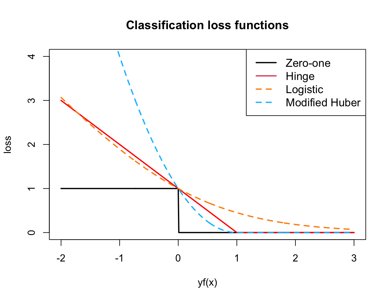
Zero-one loss is the target, but it is discontinuous and nonconvex. Hinge, logistic, and modified Huber are convex surrogates and are much easier to optimize. Logistic and modified Huber are differentiable, so gradient methods apply directly and can be attractive when \(n\) is large.
The contrast with the previous chapter is useful here. Logistic loss is (up to constants) the negative log-likelihood of a Bernoulli model, so we can map \(\hat f\) to \(\widehat{P}(Y=1\mid X=x)\) by the logistic transform. Hinge loss only cares that \(yf(x)\) be at least \(1\); once a point is beyond the margin it costs nothing further. That is why an SVM is a classifier and not, by itself, a probability model.
A nonlinear SVM with hinge loss solves \[ \min_{f\in\mathcal{H}_K} \sum_{i=1}^{n}\bigl(1-y_i f(x_i)\bigr)_+ + \lambda\|f\|_{\mathcal{H}_K}^2, \] where \(\mathcal{H}_K\) is the RKHS of the kernel \(K\). By the representer theorem the solution has the form \[ \hat f(x)=\alpha_0+\sum_{i=1}^{n}\alpha_i K(x,x_i). \] The problem reduces to an optimization over \(\alpha\in\mathbb{R}^n\), \[ \sum_{i=1}^{n} L\bigl(y_i,\ K_i^T\alpha\bigr) + \lambda\,\alpha^T K\alpha, \] where \(K\) is the \(n\times n\) kernel matrix and \(K_i\) is its \(i\)th column. If \(L\) is differentiable this is an unconstrained smooth problem.
In this view a kernel SVM first builds \(n\) new predictors, each measuring similarity to one training point, and then fits a linear model in those predictors with an \(\ell_2\)-type penalty \(\alpha^T K\alpha\).
Two restrictions of the classical SVM are worth questioning once we adopt the loss-plus-penalty view:
- The penalty on \(\alpha\) is a ridge (RKHS-norm) penalty. A lasso-type penalty on \(\alpha\) would produce a sparser expansion, using fewer kernel centers.
- The kernel is required to be positive semidefinite. Many useful similarity functions are not.
Relaxing either condition takes us outside the textbook definition of an SVM, but the resulting kernel machines are often useful supervised learning methods.
When an SVM is the wrong tool
An SVM is a strong binary classifier. It is not a default replacement for logistic regression or DA.
- It does not produce \(\widehat{P}(Y=1\mid X)\) without an extra calibration step (Platt scaling and relatives). If the scientific target is a probability, start with logistic regression.
- Multiclass problems are handled by one-versus-one or one-versus-rest reductions. That works, but it is bolted on; there is no single native multiclass hinge in the same way that multinomial logistic regression is native.
- When \(n\) is large or \(p\) is huge and sparsity in the original features is the point, \(\ell_1\)-penalized logistic regression is often the simpler statistical and computational story. The SVM sparsity is in the \(\alpha_i\) (support vectors), not in the coordinates of \(x\).
- A radial kernel with a poorly chosen width will look excellent on the training plot and fail on a new draw. Scale the features, and treat \(C\) and the kernel width as tuning parameters chosen by prediction error, not by how pretty the decision regions are.
Use an SVM when you want a flexible decision boundary and you are willing to treat \(f(x)\) as a score rather than a probability. Use logistic regression or DA when the probability model, or the linear structure in \(x\), is the object of interest.