12.3 Hierarchical Clustering
Choosing the number of clusters \(K\) may be difficult. In a Hierarchical Representation each cluster contains a single observation at the lowest level, and there is only one cluster containing all observations at the highest level. We then use a dendrogram to display the clustering result.
Hierarchical Clustering Example
Suppose we have a set of six observations:
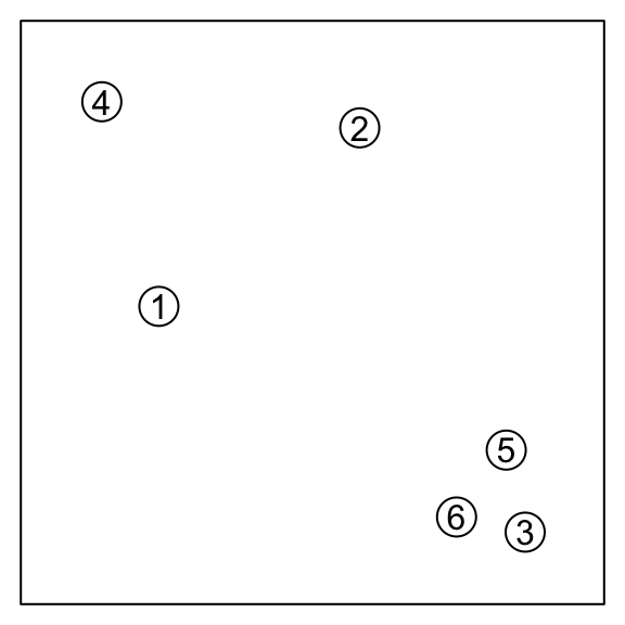
The goal is to progressively group them together until there is only one group.
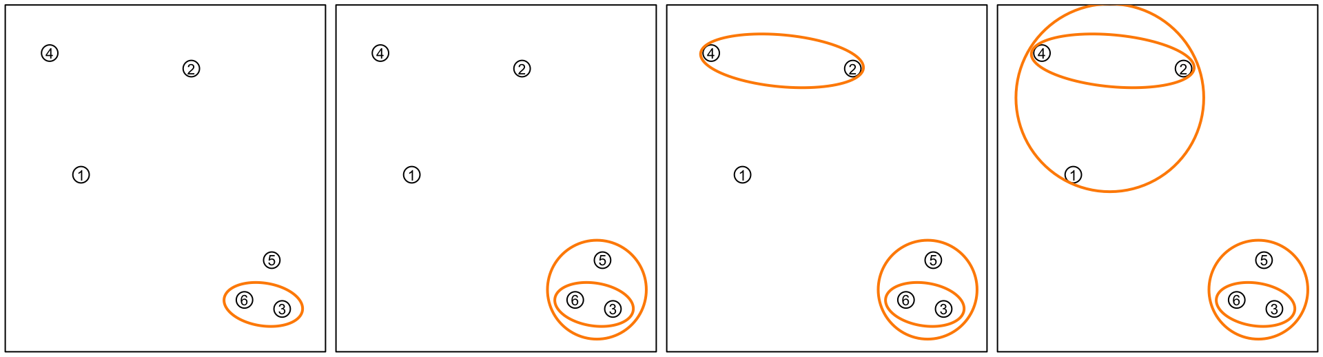
During this entire process, only the pair-wise distances are used to determine which observations are grouped. Hence, the R function hclust() will take a distance matrix and perform the clustering. A distance matrix is an \(n \times n\) matrix. As a default, we can use the Euclidean distance.
##          1         2         3         4         5         6
## 1 0.000000 1.2294164 1.7864196 1.1971565 1.4246185 1.5698349
## 2 1.229416 0.0000000 2.3996575 0.8727261 1.9243764 2.2708670
## 3 1.786420 2.3996575 0.0000000 2.8586738 0.4782442 0.2448835
## 4 1.197156 0.8727261 2.8586738 0.0000000 2.4219048 2.6741260
## 5 1.424618 1.9243764 0.4782442 2.4219048 0.0000000 0.4204479
## 6 1.569835 2.2708670 0.2448835 2.6741260 0.4204479 0.0000000
We then use this distance matrix in the hierarchical clustering algorithm.
##          1         2         3         4         5         6
## 1 0.000000 1.2294164 1.7864196 1.1971565 1.4246185 1.5698349
## 2 1.229416 0.0000000 2.3996575 0.8727261 1.9243764 2.2708670
## 3 1.786420 2.3996575 0.0000000 2.8586738 0.4782442 0.2448835
## 4 1.197156 0.8727261 2.8586738 0.0000000 2.4219048 2.6741260
## 5 1.424618 1.9243764 0.4782442 2.4219048 0.0000000 0.4204479
## 6 1.569835 2.2708670 0.2448835 2.6741260 0.4204479 0.0000000
# pass the distance matrix to hclust() we use a complete
# link function
hcfit <- hclust(dist(x), method = "complete")
par(mar = c(2, 2, 2, 1))
plot(hcfit)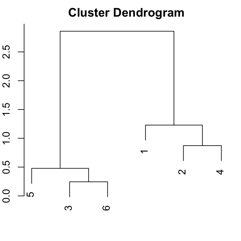
Hence, the merging process is exactly the same as we demonstrated previously. The height of each split represents how separated the two subsets are. Selecting the number of clusters is still a tricky problem. Usually, we pick a cutoff where the height of the next split is short. Hence, the above example fits well with two clusters.
An agglomerative algorithm is a bottom-up approach:
Begin with every observation representing a singleton cluster.
At each step, merge two closest clusters into one cluster and reduce the number of clusters by one.
Stop when all observations are in the same cluster.
To choose which two clusters to merge, we need (i) a distance measure between any two observations \(d(x_i, x_j)\), and (ii) a distance measure between any two sets of observations \(d(G, H)\).
A Distance \(d(G, H)\) between two clusters \(G\) and \(H\) defined as:
Complete Linkage: the furthest pair \[d(G, H) = \max_{i\in G,\, i'\in H} d_{ii'}\]
Single Linkage: the closest pair \[d(G, H) = \min_{i\in G,\, i'\in H} d_{ii'}\]
Average Linkage: average dissimilarity \[d(G, H) = \frac{1}{n_G n_H} \sum_{i\in G} \sum_{i'\in H} d_{ii'}\]
Ward Linkage: merge the pair of clusters whose combination increases the within-cluster sum of squares the least. This linkage is the closest hierarchical analogue of the \(K\)-means objective.
Different choices may result in different hierarchical structures.
To perform a hierarchical clustering, a matrix of all the pair-wise distances is sufficient, and we do not need to know the values of the original observations. This is an \(n \times n\) matrix: the \((i, i')\) element represents the distance between \(x_i\) and \(x_{i'}\). This matrix is also called a dissimilarity matrix. This is a symmetric matrix with diagonal elements that are zero.