8.1 Fitting a Logistic Regression Model
Logistic regression starts by directly modeling the conditional probability \[\eta(x) = P(Y=1 \mid X=x),\] where \(\eta(x)\) is a function bounded in \([0,1]\).
Specifically, consider a link function \(g\) that maps \(\eta(x)\) into \((-\infty, \infty)\), i.e. \[g\bigl(\eta(x)\bigr) = \mathbf{x}^T \beta.\]
Based on this formulation, the response \(Y\) conditional on \(X\) follows a Bernoulli distribution:
\[P(Y = y_i \mid X=x_i) = \eta(x_i)^{y_i} \bigl(1- \eta(x_i)\bigr)^{1-y_i},\] where \[\eta(x) = P(Y=1 \mid X=x) \quad \text{and} \quad 1-\eta(x) = P(Y=0 \mid X=x).\]
For logistic regression, we use the logit link, defined by
\[\begin{align*} \log \frac{\eta(x)}{1-\eta(x)} = x^T \beta \quad\Leftrightarrow\quad \eta(x) = \frac{\exp (x^T \beta)}{1 + \exp (x^T \beta)}. \end{align*}\] The quantity \(\log\frac{\eta(x)}{1-\eta(x)}\) is called the log-odds, and we model it as a linear function of \(x\).
8.1.1 Maximum Likelihood Approach
At each data point we observe \((x_i, y_i)\), and we want to use these pairs to estimate \(\eta(x)\), or equivalently \(\beta\). Instead of minimizing a squared-error loss, as we did for a continuous response, we follow a maximum likelihood approach.
Maximum likelihood estimation is a method that provides the most likely value of a parameter, given the data we observed. In a parametric framework, the likelihood is a function of the model parameters and the data, and the maximum likelihood estimator is obtained by maximizing the likelihood with respect to the parameters.
Recall that, conditionally on \(X\), the response \(Y\) follows a Bernoulli distribution with probability \(\eta(x)\). Therefore, the likelihood function is \[\begin{align*} \mathcal{L}(\beta \mid \mathbf{y}, \mathbf{x}) &= \prod_{i=1}^{n} p(y_i \mid x_i, \beta)\\ &= \prod_{i=1}^{n} \eta(x_i)^{y_i} \bigl(1-\eta(x_i)\bigr)^{1-y_i}. \end{align*}\] To fit the logistic regression model, we maximize the likelihood with respect to \(\beta\): \[\max_{\beta} \mathcal{L}(\beta \mid \mathbf{y}, \mathbf{x}). \]
This is equivalent to maximizing the log of the likelihood, the log-likelihood function: \[\begin{align*} \ell (\beta \mid \mathbf{y}, \mathbf{x}) &= \sum_{i=1}^{n} \log \Bigl\{\eta(x_i)^{y_i} \bigl(1-\eta(x_i)\bigr)^{1-y_i} \Bigr\}\\ &= \sum_{i=1}^{n} \Biggl\{ y_i \log \frac{\eta(x_i)}{1- \eta(x_i)} + \log \bigl(1-\eta(x_i)\bigr)\Biggr\}. \end{align*}\]
Recall that we defined \[\log \frac{\eta(x)}{1-\eta(x)} = x^T \beta.\]
Combining the expressions above, after a few lines of algebra, the log-likelihood becomes \[\ell (\beta \mid \mathbf{y}, \mathbf{x}) = \sum_{i=1}^{n}\Bigl\{ y_i x_i^T \beta - \log \bigl(1+ \exp(x_i^T \beta) \bigr)\Bigr\},\]
and the maximum likelihood estimator (MLE) \(\hat{\beta}\) is obtained by maximizing \[\max_{\beta} \ell (\beta \mid \mathbf{y}, \mathbf{x}) = \max_{\beta} \sum_{i=1}^{n}\Bigl\{ y_i x_i^T \beta - \log \bigl(1+ \exp(x_i^T \beta) \bigr)\Bigr\}.\]
Note that \(\beta\) is a vector, so we compute the gradient \(\frac{\partial \ell(\beta \mid \mathbf{y}, \mathbf{x})}{\partial \beta}\), set it equal to \(0\), solve for \(\beta\), and check the Hessian \(\frac{\partial^2 \ell(\beta \mid \mathbf{y}, \mathbf{x})}{\partial \beta \partial \beta^T}\) to confirm that the critical point is a maximum.
Solving for the MLE
Differentiating with respect to \(\beta\) and using the chain rule, the gradient is
\[\begin{align*} \frac{\partial \ell(\beta \mid \mathbf{y}, \mathbf{x})}{\partial \beta} &= \sum_{i=1}^{n} \frac{\partial }{\partial \beta} \bigl( y_i x_i^T \beta \bigr) - \frac{\partial }{\partial \beta} \Bigl(\log \bigl(1+ \exp(x_i^T \beta) \bigr) \Bigr)\\ &= \sum_{i=1}^{n} y_i x_i^T - \sum_{i=1}^{n} \frac{1}{1+ \exp(x_i^T \beta) } \cdot \frac{\partial }{\partial \beta} \bigl( 1+ \exp(x_i^T \beta) \bigr)\\ &= \sum_{i=1}^{n} y_i x_i^T - \sum_{i=1}^{n} \frac{1}{1+ \exp(x_i^T \beta) } \cdot \exp(x_i^T \beta)\, x_i^T\\ &= \sum_{i=1}^{n} y_i x_i^T - \sum_{i=1}^{n} \frac{\exp(x_i^T \beta) \, x_i^T}{1+ \exp(x_i^T \beta) }. \end{align*}\]
To obtain the Hessian, we differentiate again with respect to \(\beta\), again using the chain rule:
\[\begin{align*} \frac{\partial^2 \ell(\beta \mid \mathbf{y}, \mathbf{x})}{\partial \beta \partial \beta^T} &= \sum_{i=1}^{n} \frac{\partial }{\partial \beta} y_i x_i^T - \frac{\partial }{\partial \beta} \Biggl(\frac{\exp(x_i^T \beta) \, x_i^T}{1+ \exp(x_i^T \beta)} \Biggr) \\ &= - \sum_{i=1}^{n} \frac{\partial }{\partial \beta} \Biggl(\frac{\exp(x_i^T \beta) \, x_i^T}{1+ \exp(x_i^T \beta)} \Biggr) \\ &= - \sum_{i=1}^{n} \frac{\partial }{\partial (\exp(x_i^T \beta)) } \Biggl(\frac{\exp(x_i^T \beta) \, x_i^T}{1+ \exp(x_i^T \beta)} \Biggr) \frac{\partial \bigl(\exp(x_i^T \beta)\bigr) }{\partial \beta} \\ &= - \sum_{i=1}^{n} x_i \frac{\exp (x_i^T \beta)}{1 + \exp (x_i^T \beta)} \frac{1}{1 + \exp (x_i^T \beta)} x_i^T\\ &= - \sum_{i=1}^{n} x_i \eta(x_i) \bigl( 1- \eta(x_i) \bigr) x_i^T. \end{align*}\]
Finally, we have
- Gradient vector
\[\frac{\partial \ell(\beta \mid \mathbf{y}, \mathbf{x})}{\partial \beta} = \sum_{i=1}^{n} y_i x_i^T - \sum_{i=1}^{n} \frac{\exp(x_i^T \beta) \, x_i^T}{1+ \exp(x_i^T \beta) } = \mathbf{X}^T (\mathbf{y} - \mathbf{p}),\] where \[p_i = \eta(x_i) = P(Y=1 \mid X=x_i).\]
- Hessian matrix
\[\frac{\partial^2 \ell(\beta \mid \mathbf{y}, \mathbf{x})}{\partial \beta \partial \beta^T} = - \sum_{i=1}^{n} x_i \eta(x_i) \bigl( 1- \eta(x_i) \bigr)x_i^T = - \mathbf{X}^T \mathbf{W} \mathbf{X}.\]
The Hessian is negative semi-definite, so the log-likelihood is concave, and therefore any local maximum is a global maximum.
There is no closed-form expression for the MLE in logistic regression, but it can be obtained with an iterative Newton–Raphson procedure.
Newton–Raphson for the Logistic MLE
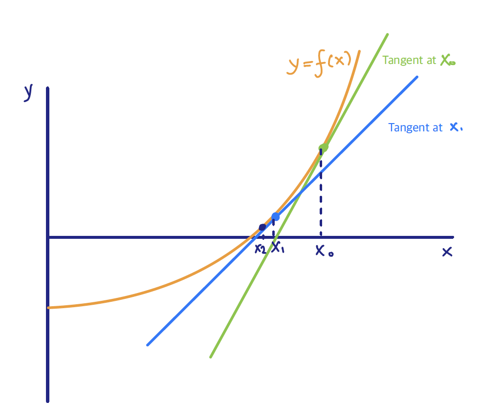
\[f(x) \approx f(x_0) + f'(x_0) (x-x_0) \] \[\Longrightarrow x = x_0 - \frac{f(x_0)}{f'(x_0)}\]
In our case, \[\begin{align*} \beta &= \beta_0 + \bigl(\mathbf{X}^T \mathbf{W} \mathbf{X}\bigr)^{-1} \mathbf{X}^T (\mathbf{y}-\mathbf{p})\\ &= \bigl(\mathbf{X}^T \mathbf{W} \mathbf{X}\bigr)^{-1} \mathbf{X}^T \mathbf{W} \Bigl( \mathbf{X} \beta_0 + \mathbf{W}^{-1}(\mathbf{y} - \mathbf{p}) \Bigr). \end{align*}\]
We can also obtain the logistic regression MLE via an iteratively reweighted least squares (IRLS) algorithm:
Start with some initial values \(\beta^0\).
Calculate the corresponding \(p_i^0 = \eta^0 (x_i)\) for \(i=1, \ldots, n\).
Define \(\mathbf{W} = \mathrm{diag}\bigl(p_i^0(1-p_i^0)\bigr)_{i=1}^{n}\).
Calculate \[\mathbf{z} = \mathbf{X} \beta^0 + \mathbf{W}^{-1}(\mathbf{y} - \mathbf{p}^0).\]
Update \(\beta^0 \leftarrow \beta^1\) with \[\beta^1 = \bigl(\mathbf{X}^T \mathbf{W} \mathbf{X}\bigr)^{-1} \mathbf{X}^T \mathbf{W} \mathbf{z}.\]
Iterate the above steps until convergence.