9.3 Nonlinear SVM: The Kernel Trick
In a linear SVM the decision boundaries are hyperplanes in the original input space. In many problems that is not flexible enough.
## Setting default kernel parameters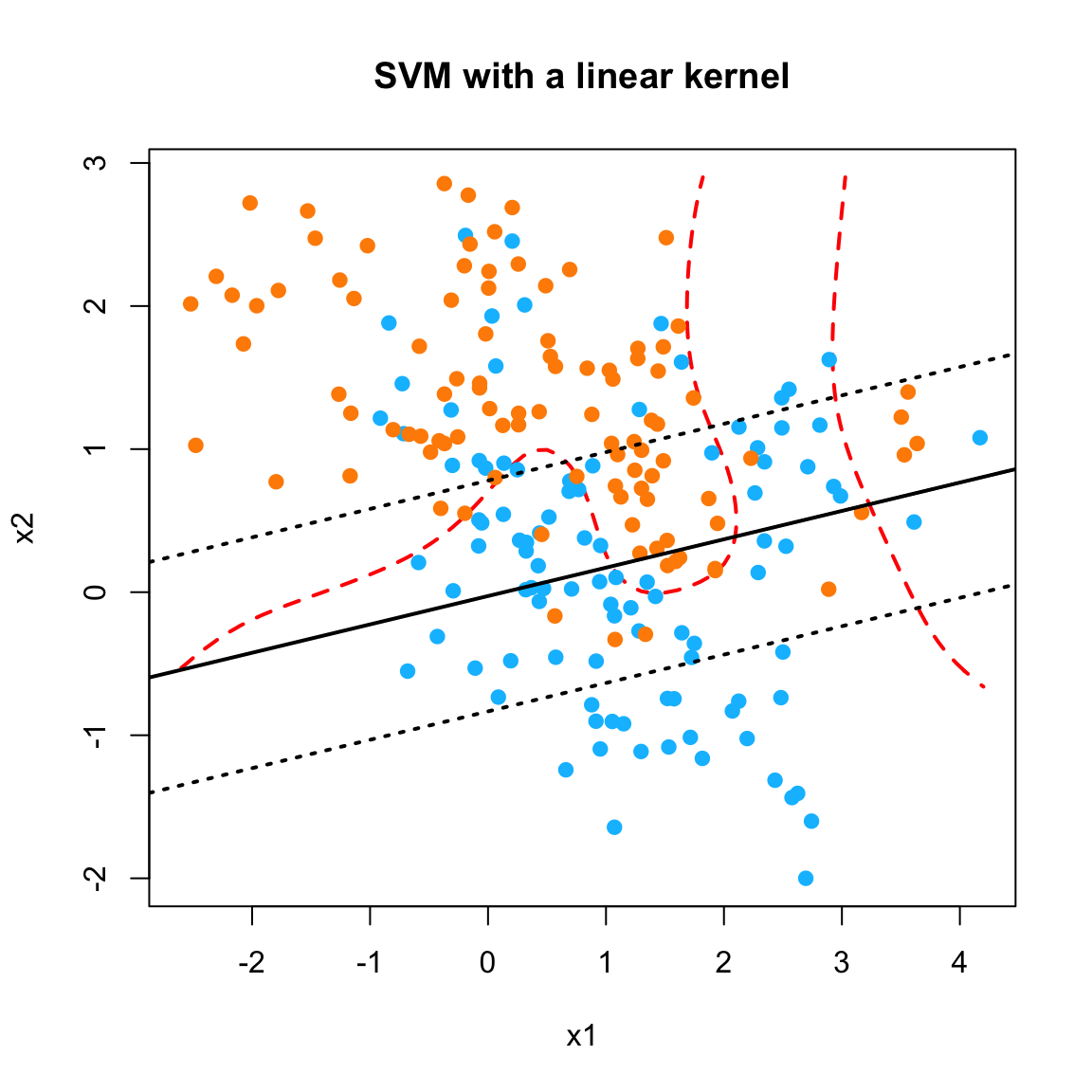
Figure 9.4: A linear SVM on a nonlinear problem (ESL mixture data)
To obtain nonlinear boundaries we enlarge the feature space with a map \[ \Phi:\mathcal{X}\to\mathcal{F},\qquad \Phi(x)=\bigl(\phi_1(x),\phi_2(x),\ldots\bigr), \] where \(\mathcal{F}\) may be finite- or infinite-dimensional, and then run a linear SVM in \(\mathcal{F}\). A linear function of \(\Phi(x)\) is typically a nonlinear function of the original \(x\). The decision function becomes \[ f(x)=\bigl\langle\Phi(x),\beta\bigr\rangle=\Phi(x)^T\beta. \]
Kernel trick
Do not compute \(\Phi(x)\) explicitly. The dual SVM depends on the data only through inner products, and \[ K(x,z)=\bigl\langle\Phi(x),\Phi(z)\bigr\rangle \] can often be evaluated directly in the original space.
Naive Approach
If \(\Phi\) were known, we could form \(\Phi(x_i)\) for each \(i\) and solve \[ \max_{\alpha} \sum_{i=1}^{n}\alpha_i - \frac12\sum_{i,j=1}^{n} y_i y_j\alpha_i\alpha_j \underbrace{\bigl\langle\Phi(x_i),\Phi(x_j)\bigr\rangle}_{=K(x_i,x_j)} \] \[ \text{subject to }\quad 0\le\alpha_i\le C,\qquad \sum_{i=1}^{n}\alpha_i y_i=0. \] The kernel trick lets us evaluate \(K(x_i,x_j)\) without ever forming \(\Phi(x_i)\).
A simple example: the homogeneous quadratic kernel \(K(x,z)=(x^T z)^2\) with \(x,z\in\mathbb{R}^p\). Let \(\Phi(x)\) collect all monomials \(x_k x_{\ell}\) for \(1\le k,\ell\le p\). Then \[\begin{align*} K(x,z) &= \Bigl(\sum_{k=1}^{p} x_k z_k\Bigr)\Bigl(\sum_{\ell=1}^{p} x_{\ell} z_{\ell}\Bigr)\\ &= \sum_{k=1}^{p}\sum_{\ell=1}^{p} (x_k x_{\ell})(z_k z_{\ell})\\ &= \bigl\langle\Phi(x),\Phi(z)\bigr\rangle. \end{align*}\] The kernel trick is useful for two reasons.
- The dual depends on the training data only through the pairwise values \(K(x_i,x_j)\). We never have to form \(\Phi(x_i)\).
- The fitted decision function can be written in terms of those same kernel evaluations, \[ f(x)=\beta_0+\sum_{i=1}^{n}\alpha_i y_i K(x,x_i) \] (or an equivalent expansion, depending on how \(\alpha\) is coded). In other words, \(\hat f\) lives in the span of \(\{K(\cdot,x_i)\}_{i=1}^{n}\).
Remark. A sufficient condition is that the kernel matrix \(\bigl(K(x_i,x_j)\bigr)\) be positive semidefinite for every finite sample. Then \(K\) is an inner product \(\langle\Phi(x),\Phi(z)\rangle\) for some feature map \(\Phi\) (Mercer’s theorem). We will use that fact and will not develop the RKHS formalism further here.
#### Computational Advantage {-}
- Evaluating \(K(x,z)=(x^T z)^2\) costs \(\mathcal{O}(p)\) operations.
- Forming \(\Phi(x)\) and \(\Phi(z)\) and then taking an inner product costs \(\mathcal{O}(p^2)\).
That is why we derived the dual: the primal is written in terms of \(\beta\in\mathcal{F}\), which we cannot even store when \(\mathcal{F}\) is infinite-dimensional, whereas the dual is written entirely in terms of \(K(x_i,x_j)\).
Common kernels
- Degree-\(d\) polynomial: \[ K(x,z)=(1+x^T z)^d \]
- Radial basis (Gaussian): \[ K(x,z)=\exp\bigl(-\|x-z\|^2/c\bigr) \]
- Sigmoid (listed for completeness; do not use it by default): \[ K(x,z)=\tanh(\gamma x^T z + r) \]
Remark. Not every function \(K\) is a valid kernel. If the kernel matrix fails to be positive semidefinite, the dual need not be convex and there may be no feature map \(\Phi\). The sigmoid kernel is a historical choice from early neural-network comparisons. It is not always positive semidefinite; prefer a polynomial or radial kernel unless you have a specific reason not to.
Remark on Convexity
Is the dual still convex after we replace \(x_i^T x_j\) by \(K(x_i,x_j)\)? The quadratic term is \[ \sum_{i,j=1}^{n} y_i y_j\alpha_i\alpha_j K(x_i,x_j) = \alpha^T \operatorname{diag}(y)\,K\,\operatorname{diag}(y)\,\alpha. \] This is a convex function of \(\alpha\) whenever \(K\) is positive semidefinite, which is the same condition that lets us treat \(K(x,z)\) as an inner product \(\langle\Phi(x),\Phi(z)\rangle\).