13.5 Hidden Markov Models
A hidden Markov model is model-based clustering in time: the observations \(X_t\) are still generated from component distributions, but the latent labels \(Z_t\) are no longer independent. They form a Markov chain, so nearby time points tend to share a cluster.
We will start by discussing an example taken from Durbin et al. (1999). A dishonest casino uses two dice, one of them is fair and the other one is biased:
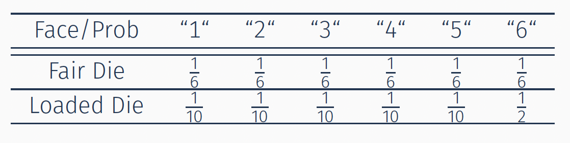
The observer does not know which die is actually taken (the state is hidden), but the sequence of throws (observations) can be used to infer which die (state) was used.
Hidden Markov Model (HMM)
A Hidden Markov Model (HMM) for \((\mathbf{Z}, \mathbf{X}) = (Z_1, \ldots, Z_n, X_1, \ldots, X_n)\) consists of
- \(X_i\)s are observed (face of a die)
- \(Z_i\)s are hidden (fair or biased)
where we assume that both \(Z\) and \(X\) are discrete random variables, taking \(m_z\) and \(m_x\) possible values, respectively.
So the HMM is parametrized by \(\theta = (w, A, B)\) where * \(w_{m_z \times 1}\): Distribution of \(Z_1\), an initial state * \(A_{m_z \times m_z}\): the transition probability matrix from \(Z_t\) to \(Z_{t+1}\) * \(B_{m_z \times m_x}\): the probability matrix (the emission distribution) for observing \(X_t\) under each hidden state \(Z_t\).
The behavior of a HMM is fully determined by the three probabilities \(w\), \(A\), and \(B\), and implicitly by \(m_z\) and \(m_x\)
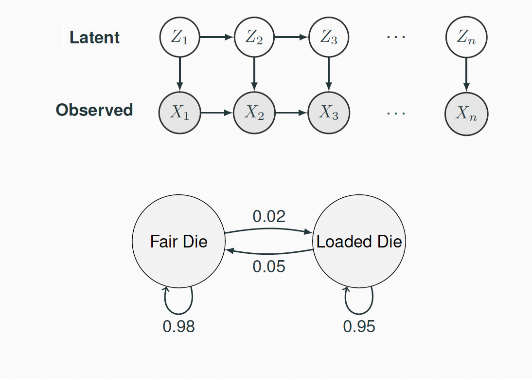
For the Dishonest Casino example, we have
- \(m_z=2\) and \(m_x=6\).
- \(A = \begin{bmatrix} 0.98 & 0.02\\ 0.05 & 0.95\end{bmatrix}\)
- \(B = \begin{bmatrix} \frac{1}{6} & \frac{1}{6} & \frac{1}{6} & \frac{1}{6} & \frac{1}{6} & \frac{1}{6} \\ \frac{1}{10} & \frac{1}{10} & \frac{1}{10} & \frac{1}{10} & \frac{1}{10} & \frac{1}{2}\end{bmatrix}\)
- \(w=(\frac{1}{2}, \frac{1}{2})\) equal probabilities if no strong prior.
We can calculate the probabilities of the observed data based on any given parameter value.
How should we model the data and detect the underlying states (which die was used)?
The underlying states \(\{Z_t; t=1, \ldots, n\}\) are a Markov chain, that satisfies the following assumptions:
Memoryless Assumption \[p(Z_t|Z_{t-1}, \ldots, Z_1) = p(Z_t|Z_{t-1})\]
Stationarity Assumption \[p(Z_t|Z_{t-1}) = p(Z_2|Z_{1})\,\,\, \text{ for } \, t=2, \ldots, n\]
The log-likelihood on the observed data is given by \[\log \left( p(\mathbf{x}|\theta) \right) = \log \left(\sum_z p(\mathbf{x}, \mathbf{z} | \theta) \right) = \log \left(\sum_z p(\mathbf{z} | \theta) p(\mathbf{x}| \mathbf{z}, \theta)\right)\] which is very hard to optimize due to the summation inside the log (generally not convex). Note that here \(\mathbf{x}\) and \(\mathbf{z}\) are the observed vectors of the sequences \(\mathbf{X}\) and \(\mathbf{Z}\), respectively. The Baum-Welch Algorithm was developed to solve this problem. It uses the EM algorithm and the Forward-Backward algorithm.
13.5.1 EM Algorithm for HMM (discrete case)
E-step: Under the current value of \(\theta\), denoted as \(\theta^{(k)}\), find \(p(\mathbf{z}|\mathbf{x}, \theta^{(k)})\), the distribution of the unobserved variables given the observed data and \(\theta^{(k)}\). Then calculate: \[\begin{align*} g(\theta) &= \mathbf{E}_{\mathbf{Z}|\mathbf{x}, \theta^{(k)}} \log p(\mathbf{x}, \mathbf{Z} | \theta) \\ &= \sum_{\mathbf{z}} P(\mathbf{Z}=\mathbf{z} |\mathbf{x}, \theta^{(k)}) \log p(\mathbf{x}, \mathbf{z} |\theta)\\ \end{align*}\]
M-step: Re-estimate the parameter \(\theta\) to maximize \(g(\theta)\): \[\theta^{(k+1)} = \arg \max_{\theta} g(\theta)\]
How to calculate \(p(\mathbf{z}|\mathbf{x}, \theta^{(k)})\) for our HMM problem?
E-step
We first write out the log-likelihood of the complete data:
\[\log p(\mathbf{z}, \mathbf{x}|\theta) = \log \Bigl (p(z_1) \prod_{t=1}^{n-1} p(z_{t+1}|z_t, \ldots, z_1, \theta) \prod_{t=1}^{n} p(x_t|z_t, \ldots, z_1, \theta) \Bigr)\]
Using the memoryless and stationarity assumptions, this can be simplified to \[\log p(\mathbf{z}, \mathbf{x}|\theta) = \log w(z_1) + \sum_{t=1}^{n-1} \log A(z_t, z_{t+1}) + \sum_{t=1}^{n} \log B(z_t, x_t)\] Note that \(\theta = (w, A, B)\). We then try to integrate it over all possible values of \(Z\), based on a current iteration value \(\theta^{(k)}\): \[E_{\mathbf{Z}|\mathbf{x}, \theta^{(k)}}\Biggl( \log p(\mathbf{x}, \mathbf{Z}|\theta ) \Biggr)\] To calculate this expectation, we need the conditional distribution of \((\mathbf{Z}|\mathbf{x}, \theta^{(k)})\) which is just the following:
\[\begin{align*} \gamma_t(i,j) &= P(Z_t=i, Z_{t+1}=j | \mathbf{X}, \theta^{(k)})\\ \gamma_t(i) &= P(Z_t=i | \mathbf{X}, \theta^{(k)}) \end{align*}\]
Suppose we already have the \(\gamma_t\) values, the E-step is \[\begin{align*} E_{\mathbf{Z}|\mathbf{x}, \theta^{(k)}}\Bigl( \log p(\mathbf{x}, \mathbf{Z}|\theta) \Bigr) &= E_{\mathbf{Z}|\mathbf{x}, \theta^{(k)}} \Bigl( \log w(Z_1) + \sum_{t=1}^{n-1} \log A(Z_t, Z_{t+1}) + \sum_{t=1}^{n} \log B(Z_t, x_t) \Bigr)\\ =& \sum_{i=1}^{m_z} \gamma_1(i) \log w(i) + \sum_{t=1}^{n-1} \sum_{i,j=1}^{m_z} \gamma_t(i,j) \log A(i,j)\\ &\quad + \sum_{t=1}^{n} \sum_{i=1}^{m_z} \gamma_t(i) \log B(i, x_t)\\ \end{align*}\] If we can compute each \(\gamma_t(i,j)\) and \(\gamma_t(i)\), this step is done.
M-step
At the M-step, we update the parameters \(\theta = (w, A, B)\) \[\begin{align*} w^{(k+1)}(i) &= \gamma_1(i), \,\,\, i=1, \ldots, m_z\\ A^{(k+1)}(i,j) &= \frac{\sum_{t=1}^{n-1} \gamma_t(i,j)}{\sum_{j'} \sum_{t=1}^{n-1} \gamma_t(i,j')}, \,\,\, i,j=1, \ldots, m_z\\ B^{(k+1)}(i,l) &= \frac{\sum_{t:x_t=l} \gamma_t(i)}{\sum_{t=1}^{n} \gamma_t(i)}, \,\,\, i=1, \ldots, m_z;\, \, l=1, \ldots, m_x \end{align*}\]
They are just the MLE estimators obtained by pooling and averaging a particular transition/emission event. For example, \(B(i, \ell)\) is observing \(X = \ell\) if the state is \(Z = i\), so we go through all events with \(Z = i\) in the entire chain, and average the events where \(X = \ell\) is observed to get the probability.
13.5.2 Forward-Backward Algorithm for HMM
In both steps, we need to calculate the conditional probabilities:
\[\gamma_t(i,j) = P(Z_t = i, Z_{t+1} = j|\mathbf{x}, \theta^{(k)})\] which is the conditional probability of transitioning from state \(i\) to state \(j\) at time point \(t\) given all the observed data \(x\), and
\[\gamma_t(i) = P(Z_t=i|\mathbf{x}, \theta^{(k)})\] the conditional probability of being at state \(i\) at time point \(t\) given all the observed data \(x\).
We will use a forward-backward algorithm to calculate this.
With no risk of ambiguity, we omit \(\theta^{(k)}\) from the notation, i.e., \(p\) is always \(p_{\theta^{(k)}}\).
For \(\gamma_t(i,j)\) by Bayes’ theorem, we have:
\[\begin{align*} \gamma_t(i,j) &= P(Z_t = i, Z_{t+1} = j |x)\\ & \propto P(X_{1:t}, Z_t=i, Z_{t+1}=j, x_{t+1}, x_{(t+2):n})\\ &= \underbrace{P(X_{1:t}, Z_t=i)}_{\alpha_t(i)} \times \underbrace{P( Z_{t+1}=j| Z_t=i)}_{A(i,j)}\\ &\quad \times \underbrace{P(x_{t+1}|Z_{t+1}=j)}_{B(j, x_{t+1})} \times \underbrace{P(x_{(t+2):n} | Z_{t+1}=j)}_{\beta_{t+1}(j)}\\ &= \alpha_t(i)\, A(i,j)\, B(j, x_{t+1})\, \beta_{t+1}(j) \end{align*}\]
where \(\alpha_t(i) = P(x_{1:t}, Z_t=i)\) is the forward probability of observing \(x_{1:t}\) and having state \(i\) at time \(t\) and \(\beta_{t+1}(j) = P(x_{(t+2):n} | Z_{t+1}=j)\) is the backward probability of observing \(x_{(t+2):n}\) given state \(j\) at time \(t\). Note that \(\alpha_t(i)\) is a joint probability, and $_{t+1}(j) $ is a conditional probability.
How to calculate \(\alpha_t(i)\) and \(\beta_{t+1}(j)\)? We do this recursively starting from the two end points \(t = 1\) and \(t = n\).
Forward Probability
For the first time point \(t=1\): \[\alpha_1(i) = P(x_1, Z_1=i) = w(i) B(i, x_1)\]
For each \(t\), we can then calculate the next time point \(\alpha_{t+1}(i)\) using the information of \(\alpha_t(i)\): \[\begin{align*} \alpha_{t+1}(i) &= P(x_1, \ldots, x_{t+1}, Z_{t+1}=i)\\ &= \sum_j P(X_1, \ldots, X_{t+1}, Z_t = j, Z_{t+1}=i)\\ &= \sum_j P(x_{1:t}, Z_t =j) p(Z_{t+1}=i|Z_t=j) P(x_{t+1}|Z_{t+1}=i)\\ &= \sum_j \alpha_t(j) A(j,i) B(i, x_{t+1}) \end{align*}\]
Backward Probability
Define \(\beta_t(i) = P(x_{(t+1):n}|Z_t=i)\). For the last time point \(t=n\) there is no future observation, so we set \[\beta_n(i)=1.\] Then we recurse backward. Using \(\beta_{t+1}\) we obtain \(\beta_t\): \[\begin{align*} \beta_t(i) &= P(x_{(t+1):n}| Z_t=i)\\ &= \sum_j P(Z_{t+1}=j | Z_t=i)\, P(x_{t+1}|Z_{t+1}=j)\, P(x_{(t+2):n}|Z_{t+1}=j)\\ &= \sum_j A(i,j)\, B(j, x_{t+1})\, \beta_{t+1}(j). \end{align*}\]
Finally, the conditional probability \(\gamma_t(i,j)\) needs to be normalized by the marginal probability to be a proper distribution:
\[\gamma_t(i,j) = \frac{\alpha_t(i) A(i,j) B(j, x_{t+1}) \beta_{t+1}(j)}{\sum_i \sum_j \alpha_t(i) A(i,j) B(j, x_{t+1}) \beta_{t+1}(j)}\] Note that this is a joint probability, so we divide by the sum of all cases. This concludes the calculation of \(\gamma_t(i,j)\)
Similarly, we can calculate \(\gamma_t(i)\) using Bayes’ Theorem \[\begin{align*} \gamma_t(i) &= P(Z_t=i|\mathbf{x})\\ &\propto P(Z_t=i,\mathbf{x})\\ &= P(Z_t=i, \mathbf{x}_{1:t}) P(\mathbf{x}_{t+1:n} |Z_t=i, \mathbf{x}_{1:t})\\ &= P(Z_t=i, \mathbf{x}_{1:t}) P(\mathbf{x}_{t+1:n} |Z_t=i)\\ &= \alpha_t(i) \beta_t(i) \end{align*}\]
Hence, after normalization, this is a proper distribution \[\gamma_t(i) = \frac{\alpha_t(i) \beta_t(i)}{\sum_i \alpha_t(i) \beta_t(i)}\]
This concludes all the components needed in the EM algorithm!