Gradient Boosting Machines in R
A GBM is a sum of trees built sequentially. For squared error (distribution = "gaussian"), tree \(t\) is fit to the current residuals and then added with a learning rate \(\lambda\):
\[ F_t(x) = F_{t-1}(x) + \lambda\,\hat h_t(x). \]
The arguments that matter for gbm are:
distribution: loss. Use"gaussian"for squared error.n.trees: number of trees \(T\) (default100). Too small underfits; too large can overfit if \(\lambda\) is not small.shrinkage: learning rate \(\lambda\) (default0.1). Smaller \(\lambda\) usually needs a largern.trees.interaction.depth: size of each tree (default1, a stump). Depth \(d\) allows interactions up to order \(d\).bag.fraction: fraction of the training rows used to fit each tree (default0.5). This is stochastic gradient boosting;1uses all rows every time.cv.folds: folds for choosingn.trees(default0, no CV error).
## Loaded gbm 2.3.1## This version of gbm is no longer under development. Consider transitioning to gbm3, https://github.com/gbm-developers/gbm3The first specification uses no shrinkage and no subsampling, so it is close to unregularized stagewise fitting. That is a poor default in practice; we use it only as a baseline.
gbm.wines = gbm(quality ~ ., data = whitewines[-test.id, ], distribution = "gaussian",
    n.trees = 100, shrinkage = 1, interaction.depth = 3, bag.fraction = 1,
    cv.folds = 5)
gbm.wines
## gbm(formula = quality ~ ., distribution = "gaussian", data = whitewines[-test.id,
## ], n.trees = 100, interaction.depth = 3, shrinkage = 1, bag.fraction = 1,
## cv.folds = 5)
## A gradient boosted model with gaussian loss function.
## 100 iterations were performed.
## The best cross-validation iteration was 8.
## There were 11 predictors of which 10 had non-zero influence.Plot the CV error against the number of trees:
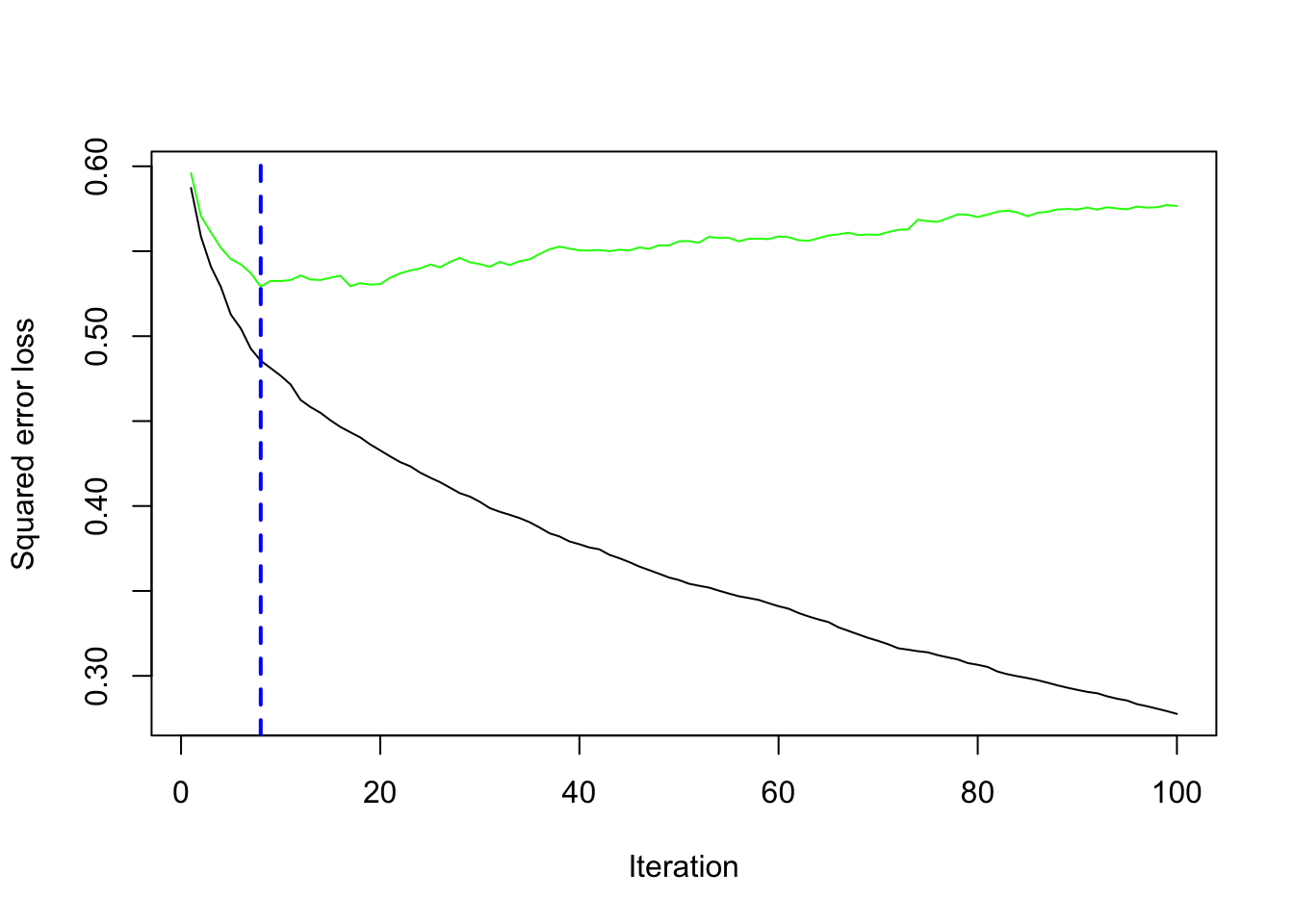
gbm.perf picks a number of trees from the CV curve. With \(\lambda=1\), that optimum is often early: later trees add little or start to overfit.
Test MSE as a function of the number of trees:
size = 1:gbm.wines$n.trees
test.err = rep(0, length(size))
for (i in 1:length(size)) {
    y.pred = predict(gbm.wines, whitewines[test.id, ], n.trees = size[i])
    test.err[i] = sum((whitewines$quality[test.id] - y.pred)^2)
}
plot(test.err, type = "n")
lines(size, test.err, lwd = 2)
abline(v = opt.size, lwd = 2, lty = 2, col = "blue")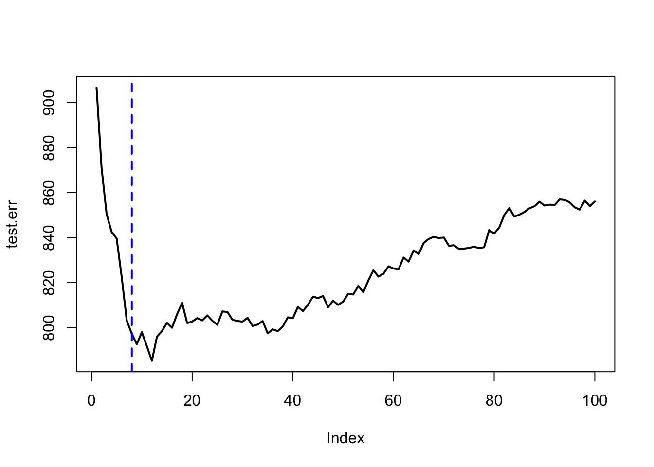
A more standard specification: small learning rate, more trees, and bag.fraction = 0.5.
gbm.wines.2 = gbm(quality ~ ., data = whitewines[-test.id, ],
    distribution = "gaussian", n.trees = 1000, shrinkage = 0.1,
    interaction.depth = 3, bag.fraction = 0.5, cv.folds = 5)

opt.size.2 = gbm.perf(gbm.wines.2)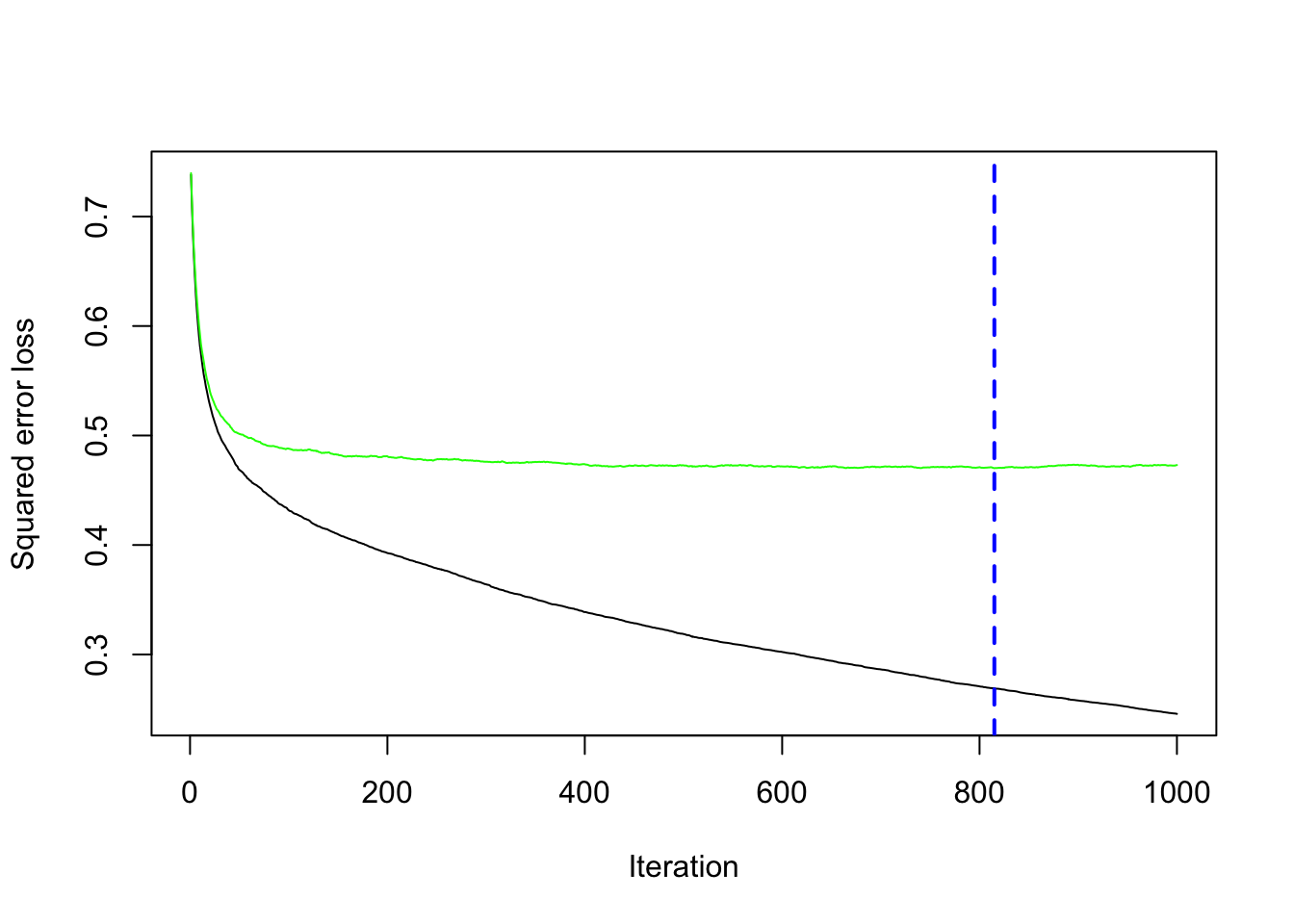
size.2 = 1:gbm.wines.2$n.trees
test.err.2 = rep(0, length(size.2))
for (i in 1:length(size.2)) {
    y.pred.2 = predict(gbm.wines.2, whitewines[test.id, ], n.trees = size.2[i])
    test.err.2[i] = sum((whitewines$quality[test.id] - y.pred.2)^2)
}
plot(test.err.2, type = "n")
lines(size.2, test.err.2, lwd = 2)
abline(v = opt.size.2, lwd = 2, lty = 2, col = "blue")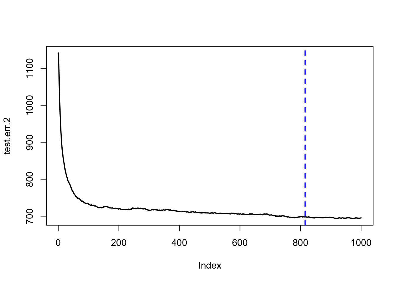
Variable importance from the baseline fit (relative influence and a permutation measure):
##                                       var   rel.inf
## alcohol                           alcohol 35.531879
## volatile.acidity         volatile.acidity 13.540395
## free.sulfur.dioxide   free.sulfur.dioxide 12.034661
## residual.sugar             residual.sugar  7.791508
## density                           density  6.230189
## total.sulfur.dioxide total.sulfur.dioxide  5.006459
## pH                                     pH  4.494230
## chlorides                       chlorides  4.058416
## fixed.acidity               fixed.acidity  3.918535
## sulphates                       sulphates  3.871500
## citric.acid                   citric.acid  3.522228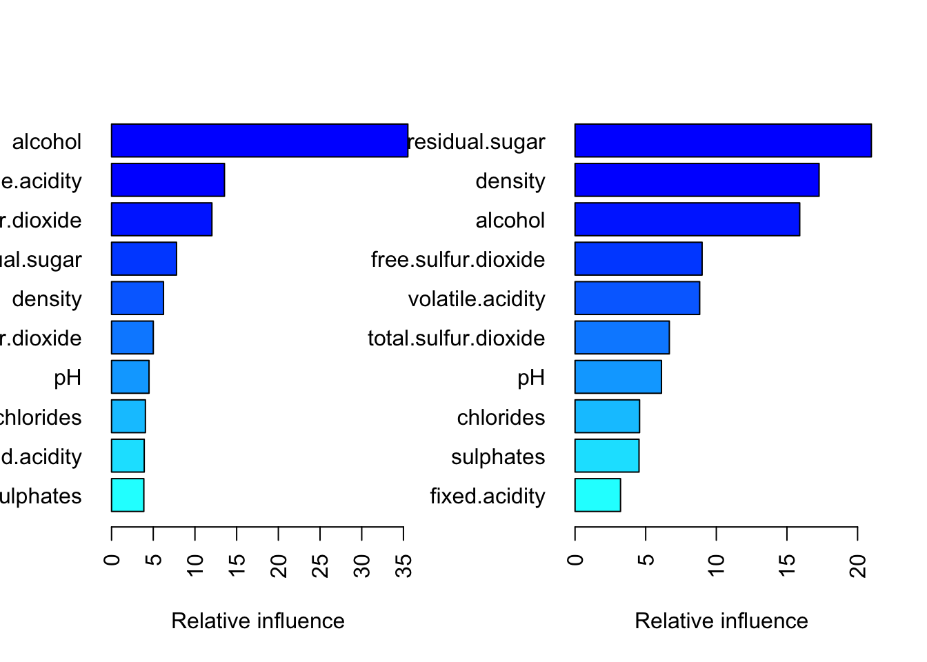
##                     var   rel.inf
## 1        residual.sugar 20.976784
## 2               density 17.275031
## 3               alcohol 15.905093
## 4   free.sulfur.dioxide  8.993392
## 5      volatile.acidity  8.822918
## 6  total.sulfur.dioxide  6.674502
## 7                    pH  6.117880
## 8             chlorides  4.568066
## 9             sulphates  4.529224
## 10        fixed.acidity  3.218505
## 11          citric.acid  2.918603