Random Forests in R
Load randomForest and hold out a test set.
## randomForest 4.7-1.2## Type rfNews() to see new features/changes/bug fixes.##
## Attaching package: 'randomForest'## The following object is masked from 'package:ggplot2':
##
## marginModel Fitting
Predict quality from every other column.
mtry is the number of variables eligible at each split.
## [1] 3Here mtry is 3, which matches the usual regression default \(\lfloor p/3 \rfloor\).
Test-set mean squared error:
yhat.test = predict(rf.wines, whitewines[test.id, ])

sum((whitewines$quality[test.id] - yhat.test)^2)/length(test.id)
## [1] 0.4129956There are two training-side errors: the error of predict() on the training rows, and the out-of-bag error stored in the forest.
yhat.train = predict(rf.wines, whitewines[-test.id, ])
sum((whitewines$quality[-test.id] - yhat.train)^2)/(n - ntest)
## [1] 0.07462265The in-sample training error is much smaller than the test error.
## [1] 0.3717869The OOB error is closer to the test error and is a more reliable estimate of generalization performance. How often each observation was left out of a bootstrap sample (first 10 rows):
## [1] 134 139 136 156 153 146 127 151 167 149
Performance vs. Number of Trees
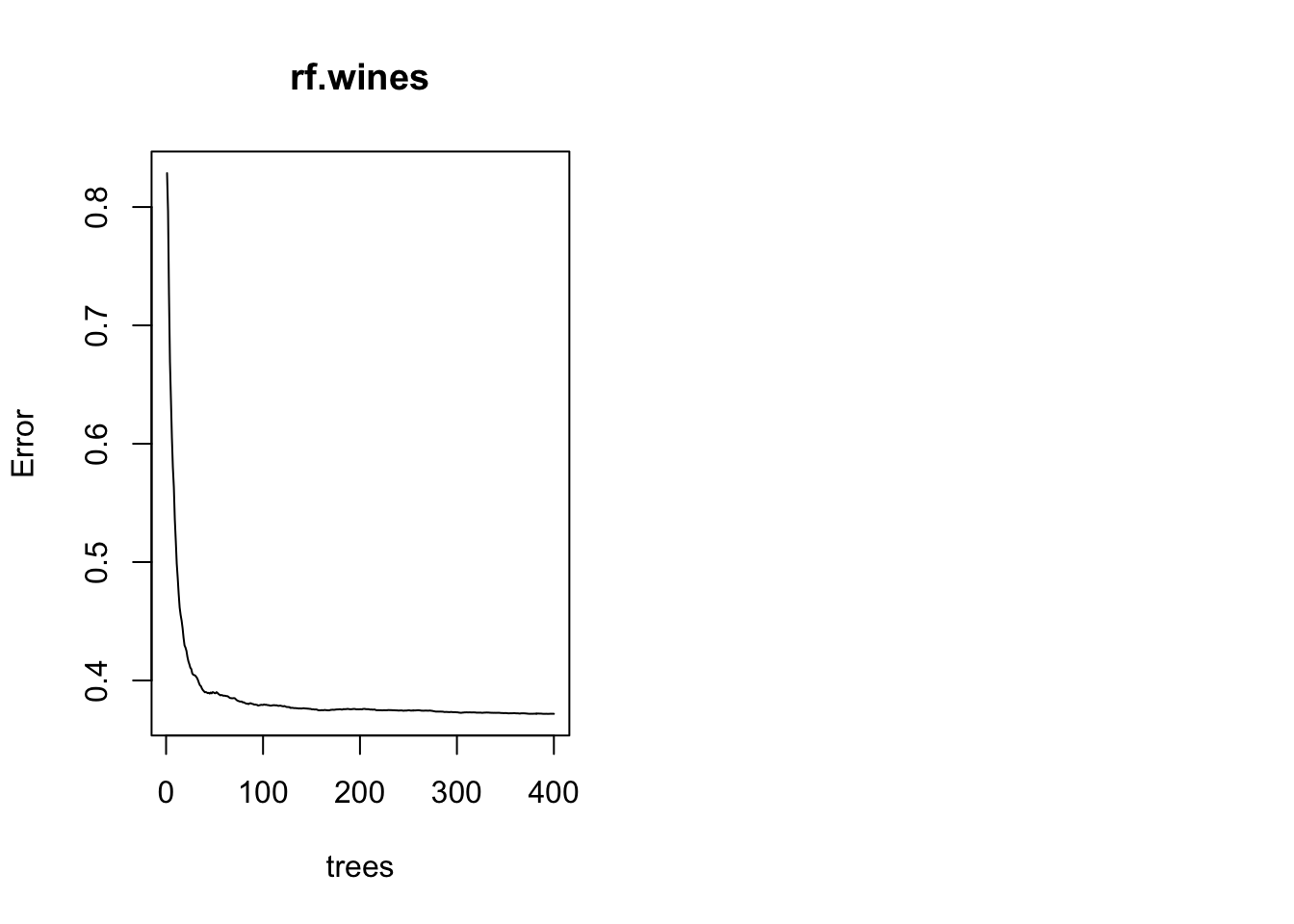
The plot is OOB MSE against the number of trees. Error usually drops quickly and then levels off. Extra trees rarely make the forest worse; they may simply be unnecessary.
Variable Importance
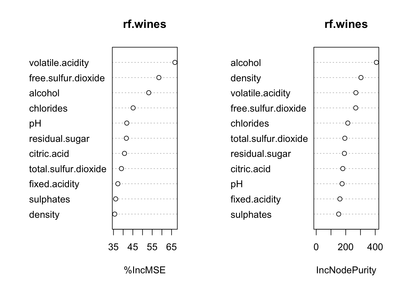
Because we set importance = TRUE, the forest stores an importance table.
##                         %IncMSE IncNodePurity
## fixed.acidity        0.06065622      160.4879
## volatile.acidity     0.17216691      268.8119
## citric.acid          0.08534572      180.0529
## residual.sugar       0.14440143      190.9511
## chlorides            0.11077918      214.0642
## free.sulfur.dioxide  0.13763805      267.8467
## total.sulfur.dioxide 0.09552685      193.8788
## density              0.24357653      303.1417
## pH                   0.08025148      175.5309
## sulphates            0.04998015      152.2842
## alcohol              0.35362770      407.9546
%IncMSE is permutation importance. IncNodePurity is the accumulated RSS gain. Scaled and unscaled versions are available, with standard errors for the permutation measure.
##                       %IncMSE IncNodePurity
## fixed.acidity        37.26205      160.4879
## volatile.acidity     66.72695      268.8119
## citric.acid          40.68951      180.0529
## residual.sugar       41.65007      190.9511
## chlorides            45.14400      214.0642
## free.sulfur.dioxide  58.44274      267.8467
## total.sulfur.dioxide 39.10194      193.8788
## density              35.64388      303.1417
## pH                   41.87941      175.5309
## sulphates            36.13850      152.2842
## alcohol              53.21555      407.9546